TL;DR: Some of my favorite arguments all following from a simple expansion of the euclidean norm and averaging.
This post is about a particular argument involving the euclidean norm. The basic idea is always the same: we expand the euclidean norm akin to the binomial formula and then do some form of averaging. We really focus on this specific argument alone here: It is not guaranteed that the estimations are optimal (although they often are) and also sometimes the argument can be generalized, replacing the euclidean norm, e.g., with the respective Bregmann divergences.
(Sub-)Gradient Descent and Online Learning
Our first example is (sub-)gradient descent without any fluff; see Cheat Sheet: Subgradient Descent, Mirror Descent, and Online Learning for a more detailed discussion and its pecularities. Consider the basic iterative scheme:
\[
\tag{subGD}
x_{t+1} \leftarrow x_t - \eta \partial f(x_t),
\]
where $f$ is a not necessarily smooth but convex function and $\partial f$ are its (sub-)gradients. We show how we can establish convergence of the above scheme to an (approximately) optimal solution $x_T$ to $\min_{x \in \RR^n} f(x)$ with $x^\esx$ being an optimal solution to $\min_{x \in \RR^n} f(x)$. To this end, we will first expand the euclidean norm as follows; basically the binomial formula:
\[\begin{align*}
\norm{x_{t+1} - x^\esx}^2 & = \norm{x_t - \eta \partial f(x_t) - x^\esx}^2 \\
& = \norm{x_t - x^\esx}^2 - 2 \eta \langle \partial f(x_t), x_t - x^\esx\rangle + \eta^2 \norm{\partial f(x_t)}^2.
\end{align*}\]
This can be rearranged to
\[\begin{align*}
\tag{subGD-iteration}
2 \eta \langle \partial f(x_t), x_t - x^\esx\rangle & = \norm{x_t - x^\esx}^2 - \norm{x_{t+1} - x^\esx}^2 + \eta^2 \norm{\partial f(x_t)}^2.
\end{align*}\]
Whenever we have an expression of the form (subGD-iteration), we can typically complete the convergence argument in three steps. We first 1) add up those expressions for $t = 0, \dots, T-1$ and 2) telescope to obtain:
\[\begin{align*}
\sum_{t = 0}^{T-1} 2\eta \langle \partial f(x_t), x_t - x^\esx\rangle & = \norm{x_0 - x^\esx}^2 - \norm{x_{T} - x^\esx}^2 + \sum_{t = 0}^{T-1} \eta^2 \norm{\partial f(x_t)}^2 \\
& \leq \norm{x_0 - x^\esx}^2 + \sum_{t = 0}^{T-1} \eta^2 \norm{\partial f(x_t)}^2.
\end{align*}\]
For simplicity, let us further assume that $\norm{\partial f(x_t)} \leq G$ for all $t = 0, \dots, T-1$ for some $G \in \RR$. Then the above simplifies to:
\[\begin{align*}
2\eta \sum_{t = 0}^{T-1} \langle \partial f(x_t), x_t - x^\esx\rangle & \leq \norm{x_0 - x^\esx}^2 + \eta^2 T G^2 \\
\Leftrightarrow \sum_{t = 0}^{T-1} \langle \partial f(x_t), x_t - x^\esx\rangle & \leq \frac{\norm{x_0 - x^\esx}^2}{2\eta} + \frac{\eta}{2} T G^2.
\end{align*}\]
At this point we could minimize the right-hand side by setting
\[\eta \doteq \frac{\norm{x_0 - x^\esx}}{G} \sqrt{\frac{1}{T}},\]
leading to
\[\begin{align*}
\sum_{t = 0}^{T-1} \langle \partial f(x_t), x_t - x^\esx\rangle & \leq G \norm{x_0 - x^\esx} \sqrt{T},
\end{align*}\]
however for this we would need to know $G$ and $\norm{x_0 - x^\esx}$, which is often not practical but we can simply set $\eta \doteq \sqrt{\frac{1}{T}}$, which is good enough, and obtain:
\[\begin{align*}
\sum_{t = 0}^{T-1} \langle \partial f(x_t), x_t - x^\esx\rangle & \leq \frac{G^2 + \norm{x_0 - x^\esx}^2}{2} \sqrt{T},
\end{align*}\]
i.e., not knowing the parameters leads to the arithmetic mean rather than the geomtric mean of the coefficients.
Then finally, 3) we average by dividing both sides by $T$. Together with convexity and the subgradient property it holds that $f(x_t) - f(x^\esx) \leq \langle \partial f(x_t), x_t - x^\esx\rangle$ and we can conclude:
\[\begin{align*}
\tag{convergenceSG}
f(\bar x) - f(x^\esx) & \leq \frac{1}{T} \sum_{t = 0}^{T-1} f(x_t) - f(x^\esx) \\
& \leq \frac{1}{T} \sum_{t = 0}^{T-1} \langle \partial f(x_t), x_t - x^\esx\rangle \\
& \leq \frac{G^2 + \norm{x_0 - x^\esx}^2}{2} \frac{1}{\sqrt{T}},
\end{align*}\]
where $\bar x \doteq \frac{1}{T} \sum_{t=0}^{T-1} x_t$ is the average of all iterates and the first inequality directly follows from convexity. As such we have effectively shown a $O(1/\sqrt{T})$ convergence rate for our subgradient descent algorithm (subGD).
It is useful to observe that the algorithm actually minimizes the average of the dual gaps at points $x_t$ given by $\langle \partial f(x_t), x_t - x^\esx\rangle$ and since the average of the dual gaps upper bounds the primal gap of the average point (via convexity) primal convergence follows. Moreover, this type of argument also allows us to obtain guarantees for online learning algorithms by simply observing that we could have used a different function $f$ for each $t$ in (subGD-iteration); for details see Cheat Sheet: Subgradient Descent, Mirror Descent, and Online Learning.
Von Neumann’s alternating projections
Next we come to von Neumann’s Alternating Projections algorithm that he formulated first in his lecture notes in 1933 and which was later (re-)printed in [vN] in 1949. Given two compact convex sets $P$ and $Q$ with associated projection operators $\Pi_P$ and $\Pi_Q$, our goal is to find a point $x \in P \cap Q$; originally von Neumann formulated the argument for linear spaces but it is pretty much immediate that his argument holds much more generally. His algorithm is quite straightforward basically, alternatingly projecting onto the respective sets:
von Neumann’s Alternating Projections [vN]
Input: Point $y_{0} \in \RR^n$, $\Pi_P$ projector onto $P \subseteq \RR^n$ and $\Pi_Q$ projector onto $Q \subseteq \RR^n$.
Output: Iterates $x_1,y_1 \dotsc \in \RR^n$
For $t = 1, \dots$ do:
$\quad x_{t+1} \leftarrow \Pi_P(y_{t})$
$\quad y_{t+1} \leftarrow \Pi_Q(x_{t+1})$
Now suppose $P \cap Q \neq \emptyset$ and let $u \in P \cap Q$ be arbitrary. We will show that the algorithm converges to a point in the intersection. The argument is quite similar to the above. We consider a given iterate, add $0$, and then use the binomial formula (and repeat):
\[\begin{align*}
\norm{y_t - u}^2 & = \norm{y_t - x_{t+1} + x_{t+1} - u}^2 = \norm{y_t - x_{t+1}}^2 + \norm{x_{t+1} - u}^2 - 2 \underbrace{\langle x_{t+1} - y_t, x_{t+1} - u \rangle}_{\leq 0} \\
& \geq \norm{y_t - x_{t+1}}^2 + \norm{x_{t+1} - u}^2 = \norm{y_t - x_{t+1}}^2 + \norm{x_{t+1} - y_{t+1} + y_{t+1} - u}^2 \\
& = \norm{y_t - x_{t+1}}^2 + \norm{x_{t+1} - y_{t+1}}^2 + \norm{y_{t+1} - u}^2 - 2 \underbrace{\langle y_{t+1} - x_{t+1} , y_{t+1} - u\rangle}_{\leq 0} \\
& \geq \norm{y_t - x_{t+1}}^2 + \norm{x_{t+1} - y_{t+1}}^2 + \norm{y_{t+1} - u}^2,
\end{align*}\]
where $\langle x_{t+1} - y_t, x_{t+1} - u \rangle \leq 0$ and $\langle y_{t+1} - x_{t+1} , y_{t+1} - u\rangle \leq 0$ are simply the first-order optimality conditions of the respective projection operator, i.e., if $x_{t+1} = \Pi_P(y_t)$ then $x_{t+1} \in \arg\min_{x \in P} \norm{x - y_t}^2$ and hence $\langle x_{t+1} - y_t, x_{t+1} - u \rangle \leq 0$ for all $u \in P$. Also observe that after a single step we obtain the inequality $\norm{y_t - u}^2 \geq \norm{y_t - x_{t+1}}^2 + \norm{x_{t+1} - u}^2$, i.e., as long as $y_t \neq x_{t+1}$, which we can safely assume as we would be done otherwise, $\norm{y_t - u}^2 > \norm{x_{t+1} - u}^2$ so that we obtain that $x_{t+1}$ moved closer to $u$ than $y_t$; similar argument is implicit for the other set.
The derivation above can be rearranged to
\[\tag{vN-iteration}
\norm{y_t - u}^2 - \norm{y_{t+1} - u}^2 \geq \norm{y_t - x_{t+1}}^2 +
\norm{x_{t+1} - y_{t+1}}^2,\]
which is similar to the iteration (subGD-iteration). As before, we can checkmate this in $3$ moves:
1) Sum up:
\[\sum_{t = 0, \dots, T-1} \left(\norm{y_t - u}^2 - \norm{y_{t+1} - u}^2\right) \geq \sum_{t = 0, \dots, T-1} \left( \norm{y_t - x_{t+1}}^2 +
\norm{x_{t+1} - y_{t+1}}^2 \right).\]
2) Telescope:
\[\norm{y_0 - u}^2 \geq \sum_{t = 0, \dots, T-1} \left( \norm{y_t - x_{t+1}}^2 +
\norm{x_{t+1} - y_{t+1}}^2\right).\]
3) Divide by $T$:
\[\frac{\norm{y_0 - u}^2}{T} \geq \frac{1}{T} \sum_{t = 0, \dots, T-1} \left( \norm{y_t - x_{t+1}}^2 +
\norm{x_{t+1} - y_{t+1}}^2 \right) \geq
\norm{x_{T} - y_{T}}^2,\]
where the last inequality is because the distances are non-increasing, so that that we can reply the average by the minimum, which is the last iterate. This shows that $\norm{x_{T} - y_{T}}^2$ goes to $0$ at a rate of $O(1/T)$, and with some minor extra reasoning we can even show that $x_T \rightarrow z$ and $y_T \rightarrow z$ with $z \in P \cap Q$.
Frank-Wolfe gap convergence in the non-convex case
The Frank-Wolfe algorithm is a first-order method that allows to optimize an $L$-smooth and convex function $f$ over a compact convex feasible region $P$, for which we have a linear minimization oracle (LMO) available, i.e., we assume that we can optimize a linear function over $P$; for more details see the two cheat sheets Cheat Sheet: Smooth Convex Optimization and
Cheat Sheet: Frank-Wolfe and Conditional Gradients. The standard Frank-Wolfe algorithm is presented below:
Frank-Wolfe Algorithm [FW] (see also [CG])
Input: Smooth convex function $f$ with first-order oracle access, feasible region $P$ with linear optimization oracle access, initial point (usually a vertex) $x_0 \in P$.
Output: Sequence of points $x_0, \dots, x_T$
For $t = 1, \dots, T$ do:
$\quad v_t \leftarrow \arg\min_{x \in P} \langle \nabla f(x_{t-1}), x \rangle$
$\quad x_{t+1} \leftarrow (1-\gamma_t) x_t + \gamma_t v_t$
A crucial characteristic of (the family of) Frank-Wolfe algorithms is that they admit a natural dual gap, the so-called Frank-Wolfe gap at any point $x \in P$, defined as $\max_{v \in P} \langle \nabla f(x), x - v \rangle$, which most algorithms also naturally compute as part of their iterations. It is straightforward to see that the Frank-Wolfe gap upper bounds the primal gap by convexity:
\[f(x) - f(x^\esx) \leq \langle \nabla f(x), x - x^\esx \rangle \leq \max_{v \in P} \langle \nabla f(x), x - v \rangle,\]
and the Frank-Wolfe gap can be “observed” compared to the primal gap, i.e., we can use it as a stopping criterion. In the case where $f$ is non-convex but smooth—our object of interest here—the Frank-Wolfe gap is still a criterion for first-order criticality, albeit not bounding the primal gap anymore and it is only necessary for global optimality but not sufficient. We want to show that the Frank-Wolfe gap converges to $0$ in the non-convex but smooth case. For this we start from the smoothness inequality—the only thing that we have in this case—and write:
\[f(x_t) - f(x_{t+1}) \geq \gamma \langle \nabla f(x_t), x_t - v_t \rangle - \gamma^2 \frac{L}{2} \norm{x_t - v_t}^2,\]
where $v_t = \arg \max_{v \in P} \langle \nabla f(x_t), x_t - v \rangle$ is the Frank-Wolfe vertex at $x_t$. Let $D$ be the diameter of $P$, so that can bound $\norm{x_t - v_t} \leq D$, for simplicity, and obtain after rearranging:
\[\tag{FWGap-iteration}
\gamma \langle \nabla f(x_t), x_t - v_t \rangle \leq f(x_t) - f(x_{t+1}) + \gamma^2 \frac{L}{2} D^2,\]
and we can continue as in (subGD-iteration): adding up, telescoping, rearranging, and simplifying leads to:
\[\sum_{t = 0, \dots, T-1} \langle \nabla f(x_t), x_t - v_t \rangle \leq \frac{f(x_0) - f(x_{T})}{\gamma} + \gamma T \frac{L}{2} D^2 \leq \frac{f(x_0) - f(x^\esx)}{\gamma} + \gamma T \frac{L}{2} D^2,\]
Dividing by $T$ and setting $\gamma \doteq \frac{1}{\sqrt{T}}$, we obtain:
\[\min_{t = 0, \dots, T-1} \langle \nabla f(x_t), x_t - v_t \rangle \leq \frac{1}{T} \sum_{t = 0, \dots, T-1} \langle \nabla f(x_t), x_t - v_t \rangle \leq \frac{f(x_0) - f(x^\esx) + \frac{LD^2}{2}}{\sqrt{T}},\]
i.e., the average of the Frank-Wolfe gaps converges to $0$ at a rate of $O(1/\sqrt{T})$ and so does the minimum.
Note. We could have chosen $\gamma$ better by minimizing the right-hand side, leading to $\gamma \doteq \sqrt{\frac{2(f(x_0) - f(x^\esx))}{LD^2 T}}$. Then we would have obtained:
\[\sum_{t = 0, \dots, T-1} \langle \nabla f(x_t), x_t - v_t \rangle \leq \frac{f(x_0) - f(x^\esx)}{\gamma} + \gamma T \frac{L}{2} D^2 = \sqrt{T} \sqrt{\frac{(f(x_0) - f(x^\esx)) LD^2}{2}},\]
and then dividing by $T$ would have given
\[\min_{t = 0, \dots, T-1} \langle \nabla f(x_t), x_t - v_t \rangle \leq \frac{1}{T} \sum_{t = 0, \dots, T-1} \langle \nabla f(x_t), x_t - v_t \rangle \leq \frac{\sqrt{\frac{(f(x_0) - f(x^\esx)) LD^2}{2}}}{\sqrt{T}}.\]
This slightly improves the constant, basically from the arithmetic mean of $f(x_0) - f(x^\esx)$ and $LD^2/2$ to the geometric mean, however at the cost or requiring prior knowledge about (or at least upper bounds on) $L$, $D$, and $f(x_0) - f(x^\esx)$.
Certifying non-membership
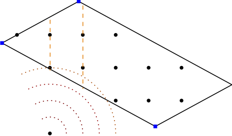
Finally, we consider the problem of certifying non-membership of a point $x_0 \not \in P$, where $P$ is a polytope that we have a linear minimization oracle (LMO) for; the same argument also works for any compact convex $P$ with LMO, however for simplicity we consider the polytopal case here.
The certificate will be a separating hyperplane, that separates $x_0$ from $P$. We apply the Frank-Wolfe algorithm to minimize the function \(f(x) = \frac{1}{2} \norm{x - x_0}^2\) over $P$, which is essentially the projection of $x_0$ onto $P$; we rescale by $1/2$ only for convenience.
Our starting point is the following expansion of the norm similar to what we have done before for von Neumann’s alternating projections. Let $v \in P$ be arbitrary and let the $x_t$ be the iterates of the Frank-Wolfe algorithm:
\[\begin{align*}
& \|x_0 -v \|^2 = \|x_0 - x_t \|^2 + \|x_t -v \|^2 - 2 \langle x_t - x_0, x_t -v \rangle \\
\Leftrightarrow\ & 2 \langle x_t - x_0, x_t -v \rangle = \|x_0 - x_t \|^2 + \|x_t -v \|^2 - \|x_0 -v \|^2 \\
\Leftrightarrow\ & \langle x_t - x_0, x_t -v \rangle = \frac{1}{2} \|x_0 - x_t \|^2 + \frac{1}{2} \|x_t -v \|^2 - \frac{1}{2} \|x_0 -v \|^2,
\end{align*}
\tag{altDualGap}\]
and observe that the left hand-side is the Frank-Wolfe gap expression at iterate $x_t$ (except for the maximization over $v \in P$) as $\nabla f(x_t) = x_t - x_0$. Let $x^* = \arg\min_{x \in P} f(x)$, i.e., the projection of $x_0$ onto $P$ under the euclidean norm.
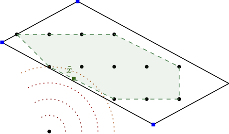
We will now derive a characterization for $x_0 \not \in P$, which also provides the certifying hyperplane.
Necessary Condition. Suppose \(\|x_t - v \| < \|x_0 - v \|\) for all vertices $v \in P$ in some iteration $t$. With this (altDualGap) reduces to
\[\tag{altTest}
\langle x_t - x_0, x_t -v \rangle < \frac{1}{2} \|x_0 - x_t \|^2,\]
for all $v \in P$ vertices. Now if we maximize over $v$ on the left-hand side in (altTest) to compute the Frank-Wolfe gap we obtain
\(\max_{v \in P} \langle x_t - x_0, x_t -v \rangle < \frac{1}{2} \|x_0 - x_t \|^2\), i.e., for all $v \in P$ (not just the vertices) it holds \(\langle x_t - x_0, x_t -v \rangle < \frac{1}{2} \|x_0 - x_t \|^2\). Plugging this back into (altDualGap), we obtain
\(\|x_t - v \| < \|x_0 - v \|\) for all $v \in P$ (not just the vertices): this will be important for the equivalence in our characterization below.
Let $v_t$ be the Frank-Wolfe vertex in iteration $t$. We then obtain:
\[\begin{align*}
\frac{1}{2} \|x_t - x_0 \|^2 - \frac{1}{2} \|x^* - x_0 \|^2 & = f(x_t) - f(x^*) \\
& \leq \max_{v \in P} \langle \nabla f(x_t), x_t - v \rangle \\
& = \langle \nabla f(x_t), x_t - v_t \rangle \\
& = \langle x_t - x_0, x_t -v_t \rangle < \frac{1}{2} \|x_0 - x_t \|^2.
\end{align*}\]
Subtracting \(\frac{1}{2} \|x_0 - x_t \|^2\) on both sides and re-arranging yields:
\[0 < \frac{1}{2} \|x^* - x_0 \|^2,\]
which proves that $x_0 \not \in P$. Moreover, (altTest) also immediately provides a separating hyperplane: Observe that the inequality
\[\langle x_t - x_0, x_t -v \rangle < \frac{1}{2} \|x_0 - x_t \|^2,\]
is actually a linear inequality in $v$ and it holds for all $v \in P$ at stated above. However, at the same time, for the choice $v \leftarrow x_0$ the inequality is violated.
Sufficient Condition. Now suppose that in each iteration $t$ there exists a vertex $\bar v_t \in P$ (not to be confused with the Frank-Wolfe vertex), so that
\(\|x_t - \bar v_t \| \geq \|x_0 - \bar v_t \|\). In this case (altDualGap) ensures:
\[\begin{align}
\langle x_t - x_0, x_t - \bar v_t \rangle & = \frac{1}{2} \|x_0 - x_t \|^2 + \frac{1}{2} \|x_t - \bar v_t \|^2 - \frac{1}{2} \|x_0 - \bar v_t \|^2 \geq \frac{1}{2} \|x_0 - x_t \|^2.
\end{align}\]
Thus, in particular the Frank-Wolfe gap satisfies in each iteration $t$ that
\[\max_{v \in P} \langle \nabla f(x_t), x_t - v \rangle \geq \langle x_t - x_0, x_t - \bar v_t \rangle \geq \frac{1}{2} \|x_0 - x_t \|^2,\]
i.e., the Frank-Wolfe gap upper bounds the distance between the current iterate $x_t$ and point $x_0$ in each iteration. Now the Frank-Wolfe gap converges to $0$ as the algorithm progresses, with iterates $x_t \in P$, so that with the usual arguments (compactness and limits etc) it follows that $x_0 \in P$. We are basically done here, but for the sake of argument, observe that by convexity we also have
\[\max_{v \in P} \langle \nabla f(x_t), x_t - v \rangle \geq f(x_t) - f(x^\esx) = \frac{1}{2} \norm{x_t - x_0}^2 - \frac{1}{2} \norm{x^\esx - x_0}^2 \geq 0,\]
and hence $\norm{x^\esx - x_0}$ has to be $0$ also, so that $x_0 = x^\esx$.
Characterization. The following are equivalent:
- (Non-Membership) $x_0 \not \in P$.
- (Distance) there exists an iteration $t$, so that \(\|x_t - v \| < \|x_0 - v \|\) for all vertices $v \in P$.
- (FW Gap) there exists an iteration $t$, so that \(\max_{v \in P} \langle x_t - x_0, x_t -v \rangle < \frac{1}{2} \|x_0 - x_t \|^2\).
References
[vN] Von Neumann, J. (1949). On rings of operators. Reduction theory. Annals of Mathematics, 401-485. pdf
[CG] Levitin, E. S., & Polyak, B. T. (1966). Constrained minimization methods. Zhurnal Vychislitel’noi Matematiki i Matematicheskoi Fiziki, 6(5), 787-823. pdf
[FW] Frank, M., & Wolfe, P. (1956). An algorithm for quadratic programming. Naval research logistics quarterly, 3(1‐2), 95-110. pdf
]]>