Cheat Sheet: Hölder Error Bounds for Conditional Gradients
TL;DR: Cheat Sheet for convergence of Frank-Wolfe algorithms (aka Conditional Gradients) under the Hölder Error Bound (HEB) condition, or how to interpolate between convex and strongly convex convergence rates. Continuation of the Frank-Wolfe series. Long and technical.
Posts in this series (so far).
- Cheat Sheet: Smooth Convex Optimization
- Cheat Sheet: Frank-Wolfe and Conditional Gradients
- Cheat Sheet: Linear convergence for Conditional Gradients
- Cheat Sheet: Hölder Error Bounds (HEB) for Conditional Gradients
- Cheat Sheet: Subgradient Descent, Mirror Descent, and Online Learning
- Cheat Sheet: Acceleration from First Principles
My apologies for incomplete references—this should merely serve as an overview.
In this third installment of the series on Conditional Gradients, I will talk about the Hölder Error Bound (HEB) condition. This post is going to be slightly different from the previous ones, as the conditional gradients part will be basically a simple corollary to our discussion of the general (constraint or unconstrained) case here. The HEB condition is extremely useful in general for establishing converge rates and I will first talk about how it compares to, e.g., strong convexity, when it holds etc. All these aspects will be independent of Frank-Wolfe per se. Going then from the general case to Frank-Wolfe is basically a simple corollary except for some non-trivial technical challenges; but those are really just that: technical challenges.
I will stick to the notation from the first post and will refer to it frequently, so you might want to give it a quick refresher or read. As before I will use Frank-Wolfe [FW] and Conditional Gradients [CG] interchangeably.
The Hölder Error Bound (HEB) condition
We have seen that in general (without acceleration), we can obtain a rate of basically $O(1/\varepsilon)$ for the smooth and convex case and a rate of basically $O(\log 1/\varepsilon)$ in the smooth and strongly convex case. A natural question to ask is what happens inbetween these two extremes, i.e., are there functions that converge with a rate of e.g., $O(1/\varepsilon^p)$? The answer is yes and the HEB condition allows basically to smoothly interpolate between the two regimes, depending on the property of the function under consideration of course.
For the sake of continuity we work here assuming the constraint case as we will aim for applications to Frank-Wolfe later, however the discussion holds more broadly for the unconstrained case as well; simply replace $P$ with $\RR^n$. In the following let $\Omega^\esx$ denote the set of optimal solutions to $\min_{x \in P} f(x)$ (there might be multiple) and let $f^\esx \doteq \min_{x \in P} f(x)$. In the following we will always assume that $x^\esx \in \Omega^\esx$.
Definition (Hölder Error Bound (HEB) condition). A convex function $f$ is satisfies the Hölder Error Bound (HEB) condition on $P$ with parameters $0 < c < \infty$ and $\theta \in [0,1]$ if for all $x \in P$ it holds: \[ c (f(x) - f^\esx)^\theta \geq \min_{y \in \Omega^\esx} \norm{x-y}. \]
Note that to simplify the exposition we assume here that the condition holds for all $x \in P$. Usually this is only assumed for a compact convex subset $K$ with $\Omega^\esx \subseteq K \subseteq P$, requiring an initial burn-in phase of the algorithm until the condition is satisfied; we ignore this subtlety here.
As far as I can see, basically this condition goes back to [L] and has been studied extensively since then, see e.g., [L2] and [BLO]; if anyone has more accurate information please ping me. So what this condition measures is how sharp the function increases around the (set of) optimal solution(s), which is why this condition sometimes is also referred to as sharpness condition. It is also important to note that the definition here depends on $P$ and the set of minimizers $\Omega^\esx$, whereas e.g., strong convexity is a global property of the function independent of $P$. Before delving further into HEB, we might wonder whether there are functions that satisfy this condition that are not strongly convex.
Example. A simple optimization problem with a function that satisfies the HEB condition with non-trivial parameters is, e.g., \[ \min_{x \in P} \norm{x-\bar x}_2^\alpha, \] where $\bar x \in \RR^n$ and $\alpha \geq 2$. In this case we obtain $\theta = 1/\alpha$. The function to be minimized is not strongly convex for $\alpha > 2$.
So the HEB condition is more general than strong convexity and, as we will see further below, it is also much weaker: it requires less from a given function (compared to strong convexity) and at the same time works for functions that are not covered by strong convexity.
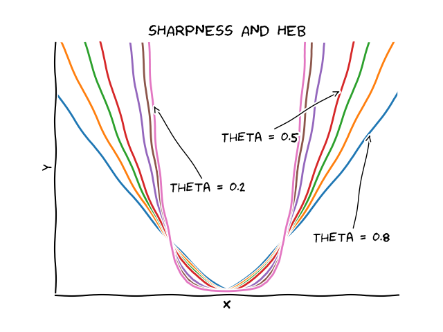
The following graph depicts functions with varying $\theta$. All functions with $\theta < 1/2$ are not strongly convex. Those with $\theta > 1/2$ are only depicted for illustration here, as they curve faster than the power of the (standard) smoothness that we use (as we will discuss briefly below) and we will be therefore limited to functions with $0 \leq \theta \leq 1/2$, where $\theta = 0$ does not provide any additional information beyond what we get from the basic convexity assumption and $\theta = 1/2$ will be essentially providing information very similar to the strongly convex case (and will lead to similar rates). If $\theta > 1/2$ is desired than the notion of smoothness has to be adjusted as well as briefly lined out in the Hölder smoothness section.
Remark (Smoothness limits $\theta$). We only consider smooth functions as we aim for applying HEB to conditional gradient methods later. This implies that the case $\theta > 1/2$ is impossible in general: suppose that $x^\esx$ is an optimal solution in the relative interior of $P$. Then $\nabla f(x^\esx) = 0$ and by smoothness we have $f(x) - f(x^\esx) \leq \frac{L}{2} \norm{x- x^\esx}^2$ and via HEB we have $\frac{1}{c^{1/\theta}} \norm{x - x^\esx}^{1/\theta} \leq f(x) - f(x^\esx)$, so that we obtain: \[\frac{1}{c^{1/\theta}} \norm{x - x^\esx}^{1/\theta} \leq f(x) - f(x^\esx) \leq \frac{L}{2} \norm{x- x^\esx}^2, \] and hence \[ K \leq \norm{x- x^\esx}^{2\theta-1} \] for some constant $K> 0$. If now $\theta > 1/2$ this inequality cannot hold as $x \rightarrow x^\esx$. However, in the non-smooth case, the HEB condition with, e.g., $\theta = 1$ might easily hold, as seen for example by choosing $f(x) = \norm{x}$. By a similar argument applied in reverse, we can see that $0 \leq \theta < 1/2$ can only be expected to hold on a bounded set in general: using $K \leq \norm{x- x^\esx}^{2\theta-1}$ from above now with $2 \theta < 1$ it follows that $\norm{x- x^\esx}^{2\theta-1} \rightarrow 0$, when $x$ follows an unbounded direction with $\norm{x} \rightarrow \infty$.
From HEB to primal gap bounds
The ultimate reason why we care for the HEB condition is that it immediately provides a bound on the primal optimality gap by a straightforward combination with convexity:
Lemma (HEB primal gap bounds). Let $f$ satisfy the HEB condition on $P$ with parameters $c$ and $\theta$. Then it holds:
\[
\tag{HEB primal bound} f(x) - f^\esx \leq c^{\frac{1}{1-\theta}} \left(\frac{\langle \nabla f(x), x - x^\esx \rangle}{\norm{x - x^\esx}}\right)^{\frac{1}{1-\theta}},
\]
or equivalently,
\[
\tag{HEB primal bound}
\frac{1}{c}(f(x) - f^\esx)^{1-\theta} \leq \frac{\langle \nabla f(x), x - x^\esx \rangle}{\norm{x - x^\esx}}
\]
for any $x^\esx \in P$ with $f(x^\esx) = f^\esx$.
Proof. By first applying convexity and then the HEB condition for any $x^\esx \in \Omega^\esx$ with $f(x^\esx) = f^\esx$ it holds:
\[\begin{align*} f(x) - f^\esx & = f(x) - f(x^\esx) \leq \langle \nabla f(x), x - x^\esx \rangle \\ & = \frac{\langle \nabla f(x), x - x^\esx \rangle}{\norm{x - x^\esx}} \norm{x - x^\esx} \\ & \leq \frac{\langle \nabla f(x), x - x^\esx \rangle}{\norm{x - x^\esx}} c (f(x) - f^\esx)^\theta, \end{align*}\]so we obtain \[ \frac{1}{c}(f(x) - f^\esx)^{1-\theta} \leq \frac{\langle \nabla f(x), x - x^\esx \rangle}{\norm{x - x^\esx}}, \] or equivalently \[ f(x) - f^\esx \leq c^{\frac{1}{1-\theta}} \left(\frac{\langle \nabla f(x), x - x^\esx \rangle}{\norm{x - x^\esx}}\right)^{\frac{1}{1-\theta}}. \] \[\qed\]
Remark (Relation to the gradient dominated property). Estimating $\frac{\langle \nabla f(x), x - x^\esx \rangle}{\norm{x - x^\esx}} \leq \norm{\nabla f(x)}$, we obtain the weaker condition: \[ f(x) - f^\esx \leq c^{\frac{1}{1-\theta}} \norm{\nabla f(x)}^{\frac{1}{1-\theta}}, \] which is known as the gradient dominated property introduced in [P]. If $\Omega^\esx \subseteq \operatorname{rel.int}(P)$, then the two conditions are equivalent and for simplicity we will use the weaker version below in our example where we show that the Scaling Frank-Wolfe algorithm adapts dynamically to the HEB bound if the optimal solution(s) are contained in the (strict) relative interior. However, if the optimal solution(s) are on the boundary of $P$ as is not infrequently the case, then the two conditions are not equivalent as $\norm{\nabla f(x)}$ might not vanish for $x \in \Omega^\esx$, whereas $\langle \nabla f(x), x - x^\esx \rangle$ does, i.e., (HEB primal bound) is tighter than the one induced by the gradient dominated property; we have seen this difference before when we analyzed linear convergence in the last post.
HEB and strong convexity
We will now show that strong convexity implies the HEB condition and then with (HEB primal bound) provides a bound on the primal gap, albeit a slightly weaker one than if we would have directly used strong convexity to obtain the bound. We briefly recall the definition of strong convexity.
Definition (strong convexity). A convex function $f$ is said to be $\mu$-strongly convex if for all $x,y \in \mathbb R^n$ it holds: \(f(y) - f(x) \geq \nabla f(x)(y-x) + \frac{\mu}{2} \norm{x-y}^2\).
Plugging in $x \doteq x^\esx$ with $x^\esx \in \Omega^\esx$ in the above, we obtain $\nabla f(x^\esx)(y-x^\esx) \geq 0$ for all $y \in P$ by first-order optimality and therefore the condition
\[ f(y) - f(x^\esx) \geq \frac{\mu}{2} \norm{x^\esx -y}^2, \]
for all $y \in P$ and rearranging leads to
\[ \tag{HEB-SC} \left(\frac{2}{\mu}\right)^{1/2} (f(y) - f(x^\esx))^{1/2} \geq \norm{x^\esx -y}, \]
for all $y \in P$, which is the HEB condition with specific parameterization $\theta = 1/2$ and $c=2/\mu$. However, here and in the HEB condition we only require this behavior around the optimal solution $x^\esx \in \Omega^\esx$ (which is unique in the case of strong convexity). The strong convexity condition is a global condition however, required for all $x,y \in \mathbb R^n$ (and not just $x = x^\esx \in \Omega^\esx$).
If we now plug-in the parameters from (HEB-SC) into (HEB primal bound), we obtain:
\[f(x) - f(x^\esx) \leq 2 \frac{\langle \nabla f(x), x - x^\esx \rangle^2}{\mu \norm{x - x^\esx}^2}.\]Note that the strong convexity induced bound obtained this way is a factor of $4$ weaker than the bound obtained in the first post in this series via optimizing out the strong convexity inequality. On the other hand we have used a simpler estimation here not relying on any gradient information as compared to the stronger bound. This weaker estimation will lead to slightly weaker convergence rate bounds: basically we lose the same $4$ in the rate.
When does the HEB condition hold
In fact, it turns out that the HEB condition holds almost always with some (potentially bad) parameterization for reasonably well behaved functions (those that we usually encounter). For example, if $P$ is compact, $\theta = 0$ and $c$ large enough will always work and the condition becomes trivial. However, HEB often also holds for non-trivial parameterization and for wide classes of functions; the interested reader is referred to [BDL] and references contained therein for an in-depth discussion. Just to give a glimpse, at the core of those arguments are variants of the Łojasewicz Inequality and the Łojasewicz Factorization Lemma.
Lemma (Łojasewicz Inequality; see [L] and [BDL]). Let $f: \operatorname{dom} f \subseteq \RR^n \rightarrow \RR$ be a lower semi-continuous and subanalytic function. Then for any compact set $C \subseteq \operatorname{dom} f$ there exist $c, \theta > 0$, so that \[ c (f(x) - f^\esx)^\theta \geq \min_{y \in \Omega^\esx} \norm{x-y}. \] for all $x \in C$.
Hölder smoothness
Without going into any detail here I would like to remark that also the smoothness condition can be weakened in a similar fashion, basically requiring (only) Hölder continuity of the gradients, i.e.,
Definition (Hölder smoothness). A convex function $f$ is said to be $(s,L)$-Hölder smooth if for all $x,y \in \mathbb R^n$ it holds: \(f(y) - f(x) \leq \nabla f(x)(y-x) + \frac{L}{s} \| x-y \|^s\).
Using this more general definition of smoothness an analogous discussion with the obvious modifications applies, e.g., now the progress guarantee from smoothness has to be adapted. The interested reader is referred to [RA] for more details and the relationship between $s$ and $\theta$.
Faster rates via HEB
We will now show how HEB can be used to obtain faster rates. We will first consider the impact of HEB from a theoretical perspective and then we will discuss how faster rates via HEB can be obtained in practice.
Theoretically faster rates
Let us assume that we run a hypothetical first-order algorithm with updates of the form $x_{t+1} \leftarrow x_t - \eta_t d_t$ for some step length $\eta_t$ and direction $d_t$. To this end, recall from the first post that the progress at some point $x$ induced by smoothness for a direction $d$ is given by (via a short step)
Progress induced by smoothness: \[ f(x_{t}) - f(x_{t+1}) \geq \frac{\langle \nabla f(x_t), d\rangle^2}{2L \norm{d}^2}, \]
and in particular for the direction pointing towards the optimal solution $d \doteq \frac{x_t - x^\esx}{\norm{x_t - x^\esx}}$ this becomes:
\[\underbrace{f(x_{t}) - f(x_{t+1})}_{\text{primal progress}} \geq \frac{\langle \nabla f(x_t), x_t - x^\esx\rangle^2}{2L \norm{x_t - x^\esx}^2}.\]At the same time, via (HEB primal bound) we have
Primal bound via HEB: \[ \frac{1}{c}(f(x_t) - f^\esx)^{1-\theta} \leq \frac{\langle \nabla f(x_t), x_t - x^\esx \rangle}{\norm{x_t - x^\esx}}. \]
Chaining these two inequalities together we obtain
\[\begin{align*} f(x_{t}) - f(x_{t+1}) & \geq \frac{\langle \nabla f(x_t), x_t - x^\esx\rangle^2}{2L \norm{x_t - x^\esx}^2} \\ & \geq \frac{\left(\frac{1}{c}(f(x_t) - f^\esx)^{1-\theta} \right)^2}{2L}. \end{align*}\]and so adding $f(x^\esx)$ on both sides and rearranging with $h_t \doteq f(x_t) - f(x^\esx)$
\[\begin{align*} h_{t+1} & \leq h_t - \frac{\frac{1}{c^2}h_t^{2-2\theta}}{2L} \\ & = h_t \left(1 - \frac{1}{2Lc^2} h_t^{1-2\theta}\right). \end{align*}\]If $\theta = 1/2$, then we obtain linear convergence with the usual arguments. Otherwise, whenever we have a contraction of the form $h_{t+1} \leq h_t \left(1 - Mh_t^{\alpha}\right)$ with $\alpha > 0$, it can be shown by induction plus some estimations that $h_t \leq O(1) \left(\frac{1}{t} \right)^\frac{1}{\alpha}$, so that we obtain
\[h_t \leq O(1) \left(\frac{1}{t} \right)^\frac{1}{1-2\theta},\]or equivalently, to achieve $h_T \leq \varepsilon$, we need roughly $T \geq \Omega\left(\frac{1}{\varepsilon^{1 - 2\theta}}\right)$.
Then, as we have done before, in an actual algorithm we use a direction $\hat d_t$ that ensures progress at least as good as from the direction $d_t = \frac{x_t - x^\esx}{\norm{x_t - x^\esx}}$ pointing towards the optimal solution by means of an inequality of the form:
\[\frac{\langle \nabla f(x_t), \hat d_t\rangle}{\norm{\hat d_t}} \geq \alpha \frac{\langle \nabla f(x_t), x_t - x^\esx\rangle}{\norm{x_t - x^\esx}},\]and the argument is for a specific algorithm is concluded as we have done before several times.
Practically faster rates
If the HEB condition almost always holds with some parameters and we generally can expect faster rates, why is it rather seldomly referred to or used (compared to e.g., strong convexity)? The reason for this is that the improved bounds are only useful in practice if the HEB parameters are known in advance, as only then we know when we can legitimately stop with a guaranteed accuracy. The key to get around this issue is to use robust restarts, which basically allow to achieve the rate implied by HEB without requiring knowledge of the parameters; this costs only a constant factor in the convergence rate compared to exactly knowing the parameters. If no error bound criterion is known, then these robust scheduled restarts rely on a grid search over a grid of logarithmic size. In the case that there is an error bound criterion available, such as e.g., the Wolfe gap in our case, then no grid search is required and basically it suffices to restart the algorithm whenever it has closed a (constant) multiplicative fraction of the residual primal gap. The overall complexity bound arises then from estimating how long each such restart takes. Coincidentally, this is exactly what the Scaling Frank-Wolfe algorithm from the first post does and we will analyze the algorithm in the next section. For details and in-depth, the interested reader is referred to [RA] for the (smooth) unconstrained case and [KDP] for the (smooth) constrained case via Conditional Gradients.
A HEB-FW for optimal solutions in relative interior
As an application of the above, we will now show that the Scaling Frank-Wolfe algorithm from the first post dynamically adjusts to the HEB condition and achieves a HEB-optimal rate up to constant factors (see p.6 of [NN] for the matching lower bound) provided that the optimal solution is contained in the strict interior of $P$; for the general case see [KDP], where we need to employ away steps. Recall from the last post, that the reason why we do not need away steps if $x^\esx \in \operatorname{rel.int}(P)$ is that in this case it holds
\[ \frac{\langle \nabla f(x),x - v\rangle}{\norm{x - v}} \geq \alpha \norm{\nabla f(x)}, \]
for some $\alpha > 0$, whenever $v \doteq \arg\min_{w \in P} \langle \nabla f(x), w \rangle$ is the Frank-Wolfe vertex and as such that the standard FW direction provides a sufficient approximation of $\norm{\nabla f(x)}$; see second post for details. This can be weakened to
\[ \tag{norm approx} \langle \nabla f(x),x - v\rangle \geq \frac{\alpha}{D} \norm{\nabla f(x)}, \]
where $D$ is the diameter of $P$, which is sufficient for our purposes in the following. From this we can derive our operational primal gap bound that we will be working with by combining (gradient norm approx) with (HEB primal bound):
\[ \tag{HEB-FW PB} f(x) - f^\esx \leq \left(\frac{cD}{\alpha}\right)^{\frac{1}{1-\theta}} \langle \nabla f(x),x - v\rangle^{\frac{1}{1-\theta}}. \]
Furthermore, let us recall the Scaling Frank-Wolfe algorithm:
Scaling Frank-Wolfe Algorithm [BPZ]
Input: Smooth convex function $f$ with first-order oracle access, feasible region $P$ with linear optimization oracle access, initial point (usually a vertex) $x_0 \in P$.
Output: Sequence of points $x_0, \dots, x_T$
Compute initial dual gap: $\Phi_0 \leftarrow \max_{v \in P} \langle \nabla f(x_0), x_0 - v \rangle$
For $t = 0, \dots, T-1$ do:
$\quad$ Find $v_t$ vertex of $P$ such that: $\langle \nabla f(x_t), x_t - v_t \rangle > \Phi_t/2$
$\quad$ If no such vertex $v_t$ exists: $x_{t+1} \leftarrow x_t$ and $\Phi_{t+1} \leftarrow \Phi_t/2$
$\quad$ Else: $x_{t+1} \leftarrow (1-\gamma_t) x_t + \gamma_t v_t$ and $\Phi_{t+1} \leftarrow \Phi_t$
As remarked earlier, the Scaling Frank-Wolfe Algorithm can be seen as a certain variant of a restart scheme, where we ‘restart’, whenever we update $\Phi_{t+1} \leftarrow \Phi_t/2$. The key is that the algorithm is parameter-free (when run with line search), does not require the estimation of HEB parameters, and is essentially optimal; skipping optimizing the update $\Phi_{t+1} \leftarrow \Phi_t/2$ with a different factor here which affects the rate only by a constant factor (in the exponent).
We will now show the following theorem, which is a straightforward adaptation from the first post incorporating (HEB-FW PB) instead of the vanilla convexity estimation.
Lemma (Scaling Frank-Wolfe HEB convergence). Let $f$ be a smooth convex function satisfying HEB with parameters $c$ and $\theta$. Then the Scaling Frank-Wolfe algorithm ensures: \[ h(x_T) \leq \varepsilon \qquad \text{for} \qquad \begin{cases} T \geq (1+K) \left(\lceil \log \frac{\Phi_0}{\varepsilon}\rceil + 1\right) & \text{ if } \theta = 1/2 \\ T \geq {\lceil \log \frac{\Phi_0}{\varepsilon}\rceil} + \frac{K 4^{-\tau}}{\left(\frac{1}{2^\tau}\right) - 1} \left(\frac{1}{\varepsilon}\right)^{-\tau} & \text{ if } \theta < 1/2 \end{cases}, \] where $K \doteq \left(\frac{cD}{2\alpha}\right)^{\frac{1}{1-\theta}} 8LD^2$, $\tau \doteq {\frac{1}{1-\theta}-2}$, and the $\log$ is to the basis of $2$.
Proof.
We consider two types of steps: (a) primal progress steps, where $x_t$ is changed and (b) dual update steps, where $\Phi_t$ is changed.
Let us start with the dual update step (b). In such an iteration we know that for all $v \in P$ it holds $\langle\nabla f(x_t),x_t - v\rangle \leq \Phi_t/2$ and in particular for $v = x^\esx$ and by (HEB-FW PB) this implies
\[h_t \leq \left(\frac{cD}{\alpha}\right)^{\frac{1}{1-\theta}} (\Phi_t/2)^{\frac{1}{1-\theta}}.\]
For a primal progress step (a), we have by the same arguments as before
\[f(x_t) - f(x_{t+1}) \geq \frac{\Phi_t^2}{8LD^2}.\]
From these two inequalities we can conclude the proof as follows: Clearly, to achieve accuracy $\varepsilon$, it suffices to halve $\Phi_0$ at most $\lceil \log \frac{\Phi_0}{\varepsilon}\rceil$ times. Next we bound how many primal progress steps of type (a) we can do between two steps of type (b); we call this a scaling phase. After accounting for the halving at the beginning of the iteration and observing that $\Phi_t$ does not change between any two iterations of type (b), by simply dividing the upper bound on the residual gap by the lower bound on the progress, the number of required steps can be at most
\[\left(\frac{cD}{\alpha}\right)^{\frac{1}{1-\theta}} (\Phi/2)^{\frac{1}{1-\theta}} \cdot \frac{8LD^2}{\Phi^2} = \underbrace{\left(\frac{cD}{2\alpha}\right)^{\frac{1}{1-\theta}} 8LD^2}_{\doteq K} \cdot \Phi^{\frac{1}{1-\theta}-2},\]
where $\Phi$ is the estimate valid for these iterations of type (a). Thus, with $\tau \doteq {\frac{1}{1-\theta}-2}$, the total number of iterations $T$ required to achieve $\varepsilon$-accuracy can be bounded by
where differentiate two cases. First let $\tau = 0$, and hence $\theta = 1/2$. This corresponds to case where we obtain linear convergence as now \[ {\lceil \log \frac{\Phi_0}{\varepsilon}\rceil} + {K \Phi_0^\tau \sum_{\ell = 0}^{\lceil \log \frac{\Phi_0}{\varepsilon}\rceil} \left(\frac{1}{2^\tau}\right)^\ell} \leq (1+K) \left(\lceil \log \frac{\Phi_0}{\varepsilon}\rceil + 1\right). \] Now let $\tau < 0$, i.e., $\theta < 1/2$. Then
\(\begin{align*} {\lceil \log \frac{\Phi_0}{\varepsilon}\rceil} + {K \Phi_0^\tau \sum_{\ell = 0}^{\lceil \log \frac{\Phi_0}{\varepsilon}\rceil} \left(\frac{1}{2^\tau}\right)^\ell} & = {\lceil \log \frac{\Phi_0}{\varepsilon}\rceil} + K \Phi_0^\tau \frac{1-\left(\frac{1}{2^\tau}\right)^{\lceil \log \frac{\Phi_0}{\varepsilon}\rceil + 1}}{1 - \left(\frac{1}{2^\tau}\right)} \\ & \leq {\lceil \log \frac{\Phi_0}{\varepsilon}\rceil} + \frac{K \Phi_0^\tau}{\left(\frac{1}{2^\tau}\right)-1} \left(\frac{1}{2^\tau}\right)^{\lceil \log \frac{\Phi_0}{\varepsilon}\rceil + 1} \\ & \leq {\lceil \log \frac{\Phi_0}{\varepsilon}\rceil} + \frac{K \Phi_0^\tau}{\left(\frac{1}{2^\tau}\right)-1} \left(\frac{4\Phi_0}{\varepsilon}\right)^{-\tau} \\ & \leq {\lceil \log \frac{\Phi_0}{\varepsilon}\rceil} + \frac{K 4^{-\tau}}{\left(\frac{1}{2^\tau}\right) - 1} \left(\frac{1}{\varepsilon}\right)^{-\tau} \end{align*}\) \[\qed\]
So we obtain the following convergence rate regimes:
- If $\theta = 1/2$, we obtain linear convergence with a convergence rate that is similar to the rate achieved in the strongly convex case up to a small constant factor, as expected from the discussion before.
- If $\theta = 0$, then $\tau = -1$ and we obtain the standard rate relying only on smoothness and convexity, namely $O\left(\frac{1}{\varepsilon^{-\tau}}\right) = O\left(\frac{1}{\varepsilon}\right)$
- If $0 < \theta < 1/2$, we have with $\tau = {\frac{1}{1-\theta}-2}$ that $0 < 2-\frac{1}{1-\theta} < 1$ and a rate of $O\left(\frac{1}{\varepsilon^{-\tau}}\right) = O\left(\frac{1}{\varepsilon^{2-\frac{1}{1-\theta}}}\right) = o\left(\frac{1}{\varepsilon}\right)$. This is strictly better than the rate obtained only from convexity and smoothness.
It is helpful to compare the rate $O\left(\frac{1}{\varepsilon^{2-\frac{1}{1-\theta}}}\right)$ with the rate $O\left(\frac{1}{\varepsilon^{1 - 2\theta}}\right)$ that we derived above directly from the contraction. For this we rewrite $2-\frac{1}{1-\theta} = \frac{1-2\theta}{1-\theta}$, so that we have $\varepsilon^{-(1 - 2\theta)}$ vs. $\varepsilon^{- \frac{1 - 2\theta}{1-\theta}}$ and maximizing out the error in the exponent over $\theta$, we obtain \(\varepsilon^{-(1 - 2\theta)} \cdot \varepsilon^{-(3-2\sqrt{2})} \geq \varepsilon^{- \frac{1 - 2\theta}{1-\theta}},\) so that the error in rate is $\varepsilon^{-(3-2\sqrt{2})} \approx \varepsilon^{-0.17157}$, which is achieved for $\theta = 1- \frac{1}{\sqrt{2}} \approx 0.29289$. This discrepancy arises from the scaling of the dual gap estimate and optimizing the factor $\gamma$ in the update $\Phi_{t+1} \leftarrow \Phi_t/\gamma$ can reduce this further to a constant factor error (rather than a constant exponent error).
Remark (Recovering the correct primal rate). As pointed out by Jannis Halbey, in the case of $\theta < 1/2$ we can immediately recover the correct primal rate from the estimation above by observing that the rate we estimated is actually for the dual gap estimator $\Phi_t$ and not for the primal gap $h_t$. As in the proof, we can use (HEB-FW PB) which implies \[h_t \leq \left(\frac{cD}{\alpha}\right)^{\frac{1}{1-\theta}} (\Phi_t/2)^{\frac{1}{1-\theta}},\] i.e., $\varepsilon_{\text{primal}} \leq O(1) \cdot \varepsilon^{\frac{1}{1-\theta}}$ and apply this to the convergence rate of the dual gap estimator to obtain: \[T \leq O\left(\frac{1}{\varepsilon^{2-\frac{1}{1-\theta}}}\right) = O\left(\frac{1}{\varepsilon^{\frac{1-2\theta}{1-\theta}}}\right) \leq O\left(\frac{1}{\varepsilon_{\text{primal}}^{1-2\theta}}\right).\] In the case where $\theta = 1/2$, the corresponding transformation is only a constant factor transformation.
Remark (HEB rates for vanilla FW). Similar HEB rate adaptivity can be shown for the vanilla Frank-Wolfe algorithm in a relatively straightforward way; e.g., a direct adaptation of the proof of [XY] will work. I opted for a proof for the Scaling Frank-Wolfe as I believe it is more straightforward and the Scaling Frank-Wolfe algorithm retains all the advantages discussed in the first post under the HEB condition.
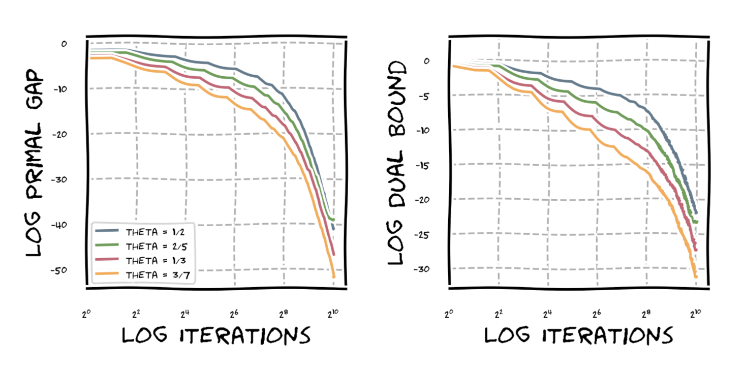
Finally, a graph showing the behavior of Frank-Wolfe under HEB on the probability simplex of dimension $30$ and function $\norm{x}_2^{1/\theta}$. As we can see, for $\theta = 1/2$, we observe linear convergence as expected, while for the other values of $\theta$ we observe various degrees of sublinear convergence of the form $O(1/\varepsilon^p)$ with $p \geq 1$. The difference in slope is not quite as pronounced as I had hoped for but, again, the bounds are only upper bounds on the convergence rates.
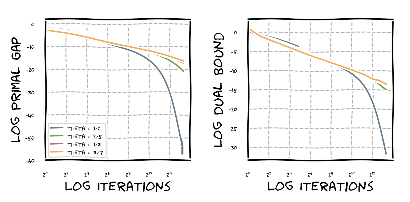
Interestingly, when using line search it seems we still achieve linear convergence and in fact the sharper functions converge faster; note this can only be a spurious phenomenon or even some bug due to the matching lower bound of our rates in [NN]. This phenomenon might be due to the fact that the progress from smoothness is only an underestimator of the achievable progress and the specific (as in simple) structure of our functions. If time permits I might try to compute out the actual optimal progress and see whether faster convergence can be proven. Here is a graph to demonstrate the difference: Frank-Wolfe run on the probability simplex for $n = 100$ and function $\norm{x}_2^{1/\theta}$.
Changelog
- 09/11/2025: Fixed two typos and added recovery of the primal rate of the Scaling Frank-Wolfe algorithm as pointed out by Jannis Halbey.
References
[CG] Levitin, E. S., & Polyak, B. T. (1966). Constrained minimization methods. Zhurnal Vychislitel’noi Matematiki i Matematicheskoi Fiziki, 6(5), 787-823. pdf
[FW] Frank, M., & Wolfe, P. (1956). An algorithm for quadratic programming. Naval research logistics quarterly, 3(1‐2), 95-110. pdf
[L] Łojasiewicz, S. (1963). Une propriété topologique des sous-ensembles analytiques réels. Les équations aux dérivées partielles, 117, 87-89.
[L2] Łojasiewicz, S. (1993). Sur la géométrie semi-et sous-analytique. Ann. Inst. Fourier, 43(5), 1575-1595. pdf
[BLO] Burke, J. V., Lewis, A. S., & Overton, M. L. (2002). Approximating subdifferentials by random sampling of gradients. Mathematics of Operations Research, 27(3), 567-584. pdf
[P] Polyak, B. T. (1963). Gradient methods for minimizing functionals. Zhurnal Vychislitel’noi Matematiki i Matematicheskoi Fiziki, 3(4), 643-653.
[BDL] Bolte, J., Daniilidis, A., & Lewis, A. (2007). The Łojasiewicz inequality for nonsmooth subanalytic functions with applications to subgradient dynamical systems. SIAM Journal on Optimization, 17(4), 1205-1223. pdf
[RA] Roulet, V., & d’Aspremont, A. (2017). Sharpness, restart and acceleration. In Advances in Neural Information Processing Systems (pp. 1119-1129). pdf
[KDP] Kerdreux, T., d’Aspremont, A., & Pokutta, S. (2018). Restarting Frank-Wolfe. pdf
[XY] Xu, Y., & Yang, T. (2018). Frank-Wolfe Method is Automatically Adaptive to Error Bound Condition. arXiv preprint arXiv:1810.04765. pdf
[BPZ] Braun, G., Pokutta, S., & Zink, D. (2017, July). Lazifying Conditional Gradient Algorithms. In International Conference on Machine Learning (pp. 566-575). pdf
[NN] Nemirovskii, A. & Nesterov, Y. E. (1985), Optimal methods of smooth convex minimization, USSR Computational Mathematics and Mathematical Physics 25(2), 21–30.
Comments