Projection-Free Adaptive Gradients for Large-Scale Optimization
TL;DR: This is an informal summary of our recent paper Projection-Free Adaptive Gradients for Large-Scale Optimization by Cyrille Combettes, Christoph Spiegel, and Sebastian Pokutta. We propose to improve the performance of state-of-the-art stochastic Frank-Wolfe algorithms via a better use of first-order information. This is achieved by blending in adaptive gradients, a method for setting entry-wise step-sizes that automatically adjust to the geometry of the problem. Computational experiments on convex and nonconvex objectives demonstrate the advantage of our approach.
Written by Cyrille Combettes.
Introduction
We consider the family of stochastic Frank-Wolfe algorithms, addressing constrained finite-sum optimization problems
\[\min_{x\in\mathcal{C}}\left\{f(x)\overset{\text{def}}{=}\frac{1}{m}\sum_{i=1}^mf_i(x)\right\},\]where $\mathcal{C}\subset\mathbb{R}^n$ is a compact convex set and $f_1,\ldots,f_m\colon\mathbb{R}^n\rightarrow\mathbb{R}$ are smooth convex functions. Their generic template is presented in Template 1. When $\tilde{\nabla}f(x_t)=\nabla f(x_t)$, we recover the original Frank-Wolfe algorithm (Frank and Wolfe, 1956), a.k.a. conditional gradient algorithm (Levitin and Polyak, 1966). It is a simple projection-free algorithm, that computes a linear minimization at each iteration and moves in the direction of the solution $v_t$ returned, with a step-size $\gamma_t\in\left[0,1\right]$ ensuring that the new iterate $x_{t+1}=(1-\gamma_t)x_t+\gamma_tv_t\in\mathcal{C}$ is feasible by convex combination. Hence, it does not need to compute projections back onto $\mathcal{C}$.
Template 1. Stochastic Frank-Wolfe
Input: Start point $x_0\in\mathcal{C}$, step-sizes $\gamma_t\in\left[0,1\right]$.
$\text{ }$ 1: $\text{ }$ for $t=0$ to $T-1$ do
$\text{ }$ 2: $\quad$ Update the gradient estimator $\tilde{\nabla}f(x_t)$
$\text{ }$ 3: $\quad$ $v_t\leftarrow\underset{v\in\mathcal{C}}{\arg\min}\langle\tilde{\nabla}f(x_t),v\rangle$
$\text{ }$ 4: $\quad$ $x_{t+1}\leftarrow x_t+\gamma_t(v_t-x_t)$
$\text{ }$ 5: $\text{ }$ end for
When $m$ is very large, querying exact first-order information from $f$ can be too expensive. Instead, stochastic Frank-Wolfe algorithms build a gradient estimator $\tilde{\nabla}f(x_t)$ with only approximate first-order information. For example, the Stochastic Frank-Wolfe algorithm (SFW) takes the average $\tilde{\nabla}f(x_t)\leftarrow(1/b_t)\sum_{i=i_1}^{i_{b_t}}\nabla f_i(x_t)$ over a minibatch $i_1,\ldots,i_{b_t}$ sampled uniformly at random from \(\{1,\ldots,m\}\). State-of-the-art stochastic Frank-Wolfe algorithms also include the Stochastic Variance-Reduced Frank-Wolfe algorithm (SVRF) (Hazan and Luo, 2016), the Stochastic Path-Integrated Differential EstimatoR Frank-Wolfe algorithm (SPIDER-FW) (Yurtsever et al., 2019; Shen et al., 2019), the Online stochastic Recursive Gradient-based Frank-Wolfe algorithm (ORGFW) (Xie et al., 2020), and the Constant batch-size Stochastic Frank-Wolfe algorithm (CSFW) (Négiar et al., 2020). Their strategies are reported in Table 1.
Table 1: Gradient estimator updates in stochastic Frank-Wolfe algorithms. The indices $i_1,\ldots,i_{b_t}$ are sampled i.i.d. uniformly at random from \(\{1,\ldots,m\}\).
| Algorithm | Update $\tilde{\nabla}f(x_t)$ in Line 2 | Additional information |
|---|---|---|
| SFW | $\displaystyle\frac{1}{b_t}\sum_{i=i_1}^{i_{b_t}}\nabla f_i(x_t)$ | $\varnothing$ |
| SVRF | \(\displaystyle\nabla f(\tilde{x}_t)+\frac{1}{b_t}\sum_{i=i_1}^{i_{b_t}}(\nabla f_i(x_t)-\nabla f_i(\tilde{x}_t))\) | $\tilde{x}_t$ is the last snapshot iterate |
| SPIDER-FW | \(\displaystyle\nabla f(\tilde{x}_t)+\frac{1}{b_t}\sum_{i=i_1}^{i_{b_t}}(\nabla f_i(x_t)-\nabla f_i(x_{t-1}))\) | $\tilde{x}_t$ is the last snapshot iterate |
| ORGFW | $\displaystyle\frac{1}{b_t}\sum_{i=i_1}^{i_{b_t}}\nabla f_i(x_t)+(1-\rho_t)\left(\tilde{\nabla}f(x_{t-1})-\frac{1}{b_t}\sum_{i=i_1}^{i_{b_t}}\nabla f_i(x_{t-1})\right)$ | $\rho_t$ is the momentum parameter |
| CSFW | \(\displaystyle\tilde{\nabla}f(x_{t-1})+\sum_{i=i_1}^{i_{b_t}}\left(\frac{1}{m}f_i'(\langle a_i,x_t\rangle)-[\alpha_{t-1}]_i\right)a_i\) and \([\alpha_t]_i\leftarrow(1/m)f_i'(\langle a_i,x_t\rangle)\) if \(i\in\{i_1,\ldots,i_{b_t}\}\) else \([\alpha_{t-1}]_i\) |
Assumes separability of $f$ as $\displaystyle f(x)=\frac{1}{m}\sum_{i=1}^mf_i(\langle a_i,x\rangle)$ |
In our paper, we propose to improve the performance of this family of algorithms by using adaptive gradients.
The Adaptive Gradient algorithm
The Adaptive Gradient algorithm (AdaGrad) (Duchi et al., 2011; McMahan and Streeter, 2010) is presented in Algorithm 2. The new iterate $x_{t+1}$ is obtained by solving a subproblem in Line 4. The default value for the offset hyperparameter is $\delta\leftarrow10^{-8}$.
Algorithm 2. Adaptive Gradient (AdaGrad)
Input: Start point $x_0\in\mathcal{C}$, offset $\delta>0$, learning rate $\eta>0$.
$\text{ }$ 1: $\text{ }$ for $t=0$ to $T-1$ do
$\text{ }$ 2: $\quad$ Update the gradient estimator $\tilde{\nabla}f(x_t)$
$\text{ }$ 3: $\quad$ $H_t\leftarrow\operatorname{diag}\left(\delta1+\sqrt{\sum_{s=0}^t\tilde{\nabla}f(x_s)^2}\,\right)$
$\text{ }$ 4: $\quad$ \(x_{t+1}\leftarrow\underset{x\in\mathcal{C}}{\arg\min}\,\eta\langle\tilde{\nabla}f(x_t),x\rangle+\frac{1}{2}\|x-x_t\|_{H_t}^2\)
$\text{ }$ 5: $\text{ }$ end for
The matrix $H_t\in\mathbb{R}^{n\times n}$ is diagonal and satisfies for all \(i,j\in\{1,\ldots,n\}\),
\[[H_t]_{i,j}=\delta+\sqrt{\sum_{s=0}^t[\tilde{\nabla}f(x_s)]_i^2}\quad\text{if }i=j\quad\text{else } 0.\]To see why AdaGrad builds entry-wise step-sizes from past first-order information, note that the subproblem in Line 4 is equivalent to
by first-order optimality condition (Polyak, 1987), where \(\|\cdot\|_{H_t}\colon u\in\mathbb{R}^n\mapsto\sqrt{\langle u,H_tu\rangle}\). Ignoring the constraint set $\mathcal{C}$ for ease of exposition, we obtain
\[x_{t+1}\leftarrow x_t-\eta H_t^{-1}\tilde{\nabla}f(x_t),\]i.e., for every feature \(i\in\{1,\ldots,n\}\),
\[[x_{t+1}]_i\leftarrow[x_t]_i-\frac{\eta[\tilde{\nabla}f(x_t)]_i}{\delta+\sqrt{\sum_{s=0}^t[\tilde{\nabla}f(x_s)]_i^2}}.\]Therefore, $\delta$ prevents from dividing by zero and the step-sizes automatically adjust to the geometry of the problem. In particular, rare but potentially very informative features do not go unnoticed as they receive a large step-size whenever they appear.
Frank-Wolfe with adaptive gradients
For constrained optimization, AdaGrad can be very expensive as it requires solving a constrained subproblem at each iteration (Line 4), which, by (1), can also be seen as a projection in the non-Euclidean norm \(\|\cdot\|_{H_t}\). Instead, we propose to solve the subproblems very incompletely, via a small and fixed number of iterations of the Frank-Wolfe algorithm. This approach is aimed at designing an efficient method in practice. In particular, contrary to Lan and Zhou (2016), we do not worry about the accuracy of the solutions to the subproblems. We present our method via a generic template in Template 3.
Template 3. Frank-Wolfe with adaptive gradients
Input: Start point $x_0\in\mathcal{C}$, number of inner iterations $K$, learning rate $\eta>0$.
$\text{ }$ 1: $\text{ }$ for $t=0$ to $T-1$ do
$\text{ }$ 2: $\quad$ Update the gradient estimator $\tilde{\nabla}f(x_t)$ $\triangleright$ as in any of Table 1
$\text{ }$ 3: $\quad$ Update the diagonal matrix $H_t$ $\triangleright$ as in, e.g., Line 3 of Algorithm 2
$\text{ }$ 4: $\quad$ \(y_0^{(t)}\leftarrow x_t\)
$\text{ }$ 5: $\quad$ for $k=0$ to $K-1$ do
$\text{ }$ 6: $\quad\quad$ \(\nabla Q_t(y_k^{(t)})\leftarrow\tilde{\nabla}f(x_t)+\frac{1}{\eta}H_t(y_k^{(t)}-x_t)\)
$\text{ }$ 7: $\quad\quad$ \(v_k^{(t)}\leftarrow\underset{v\in\mathcal{C}}{\arg\min}\langle\nabla Q_t(y_k^{(t)}),v\rangle\)
$\text{ }$ 8: $\quad\quad$ \(\gamma_k^{(t)}\leftarrow\min\left\{\eta\frac{\langle\nabla Q_t(y_k^{(t)}),y_k^{(t)}-v_k^{(t)}\rangle}{\|y_k^{(t)}-v_k^{(t)}\|_{H_t}^2},1\right\}\)
$\text{ }$ 9: $\quad\quad$ \(y_{k+1}\leftarrow y_k^{(t)}+\gamma_k^{(t)}(v_k^{(t)}-y_k^{(t)})\)
10: $\quad$ end for
11: $\quad$ \(x_{t+1}\leftarrow y_K^{(t)}\)
12: $\text{ }$ end for
Lines 4-10 apply $K$ iterations of the Frank-Wolfe algorithm on
\[\min_{x\in\mathcal{C}}\left\{Q_t(x)\overset{\text{def}}{=}f(x_t)+\langle\tilde{\nabla}f(x_t),x-x_t\rangle+\frac{1}{2\eta}\|x-x_t\|_{H_t}^2\right\},\]which is equivalent to the AdaGrad subproblem. The sequence of iterates is denoted by $y_0^{(t)},\ldots,y_K^{(t)}$, starting from $x_t=y_0^{(t)}$ and ending at $x_{t+1}=y_K^{(t)}$. In our experiments, we typically set $K\sim5$. The strategy in Line 2 can be that of any of the variants SFW, SVRF, SPIDER-FW, ORGFW, or CSFW. When using variant X, the associated method is named AdaX.
Computational experiments
We compare our method to SFW, SVRF, SPIDER-FW, ORGFW, and CSFW. For the three experiments with convex objectives, we plot our method using the best performing stochastic Frank-Wolfe variant. For the three neural network experiments, CSFW is not applicable and we run AdaSFW only, as variance reduction may be ineffective in deep learning (Defazio and Bottou, 2019). In addition, since momentum has become a key ingredient for neural network optimization, we demonstrate that AdaSFW also works very well with momentum. The method is named AdamSFW and $H_t$ is built as in Reddi et al. (2018).
The results are presented in Figure 1. One important observation is that none of the previous methods outperform the vanilla SFW on the nonconvex experiments, except on the MNIST dataset. On the IMDB dataset, AdaSFW yields the best test performance despite optimizing slowly over the training set, and AdamSFW reaches its maximum accuracy very fast which can be interesting if we consider using early stopping.
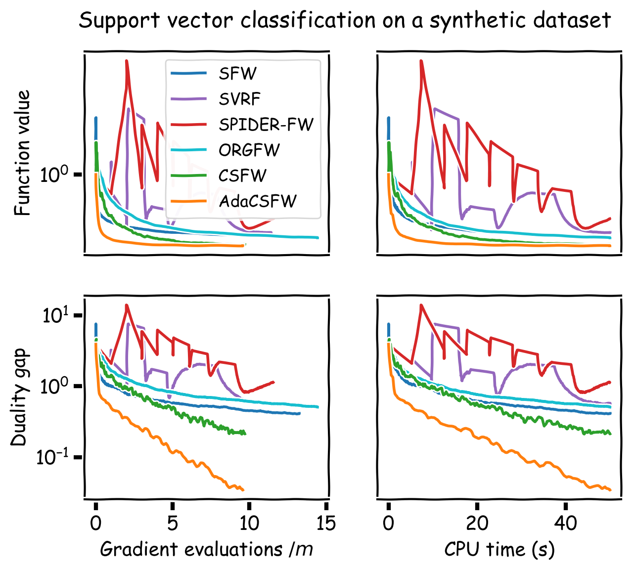
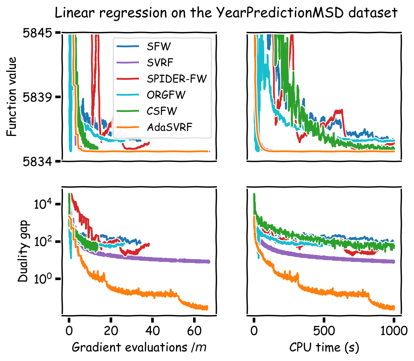
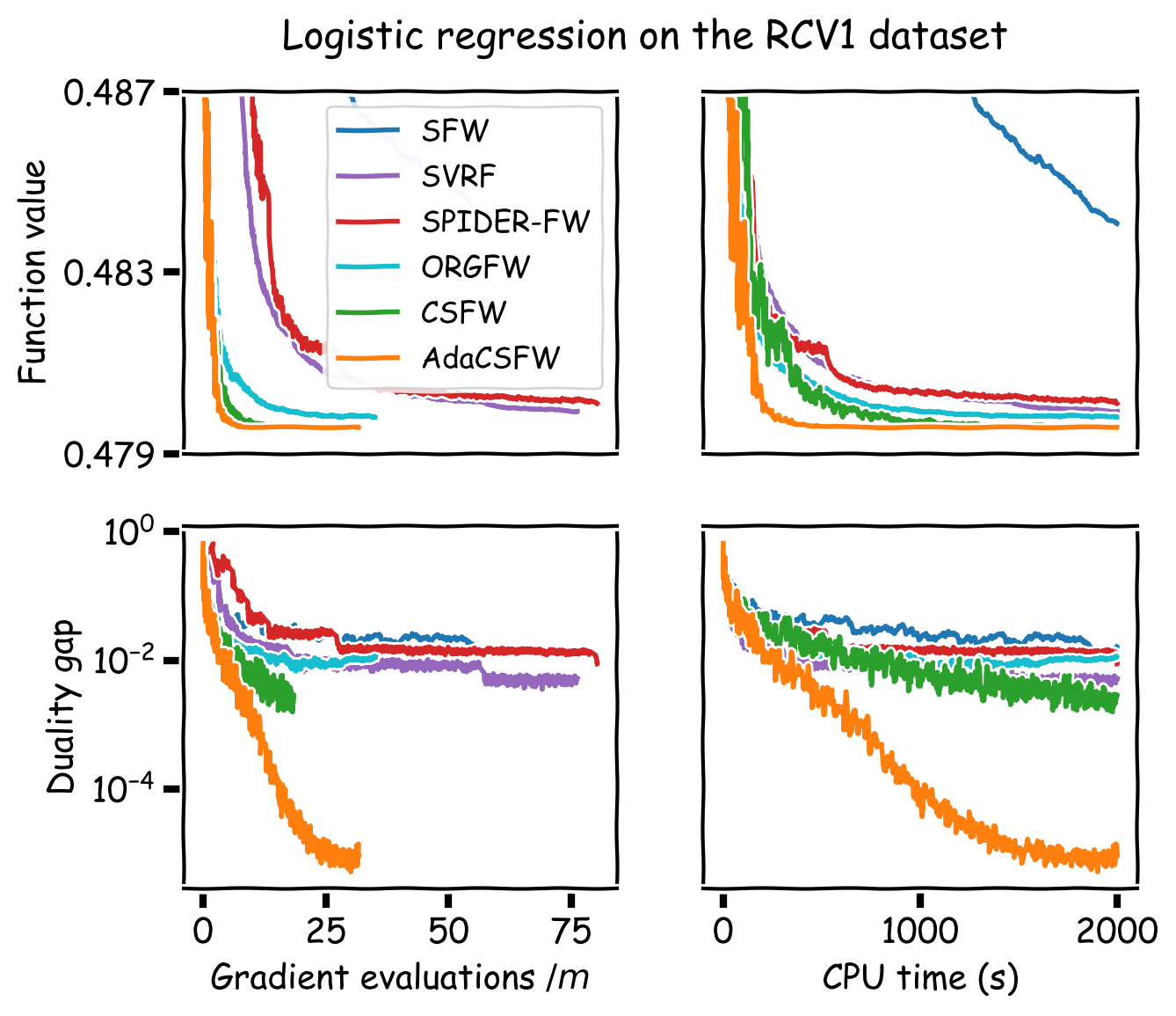
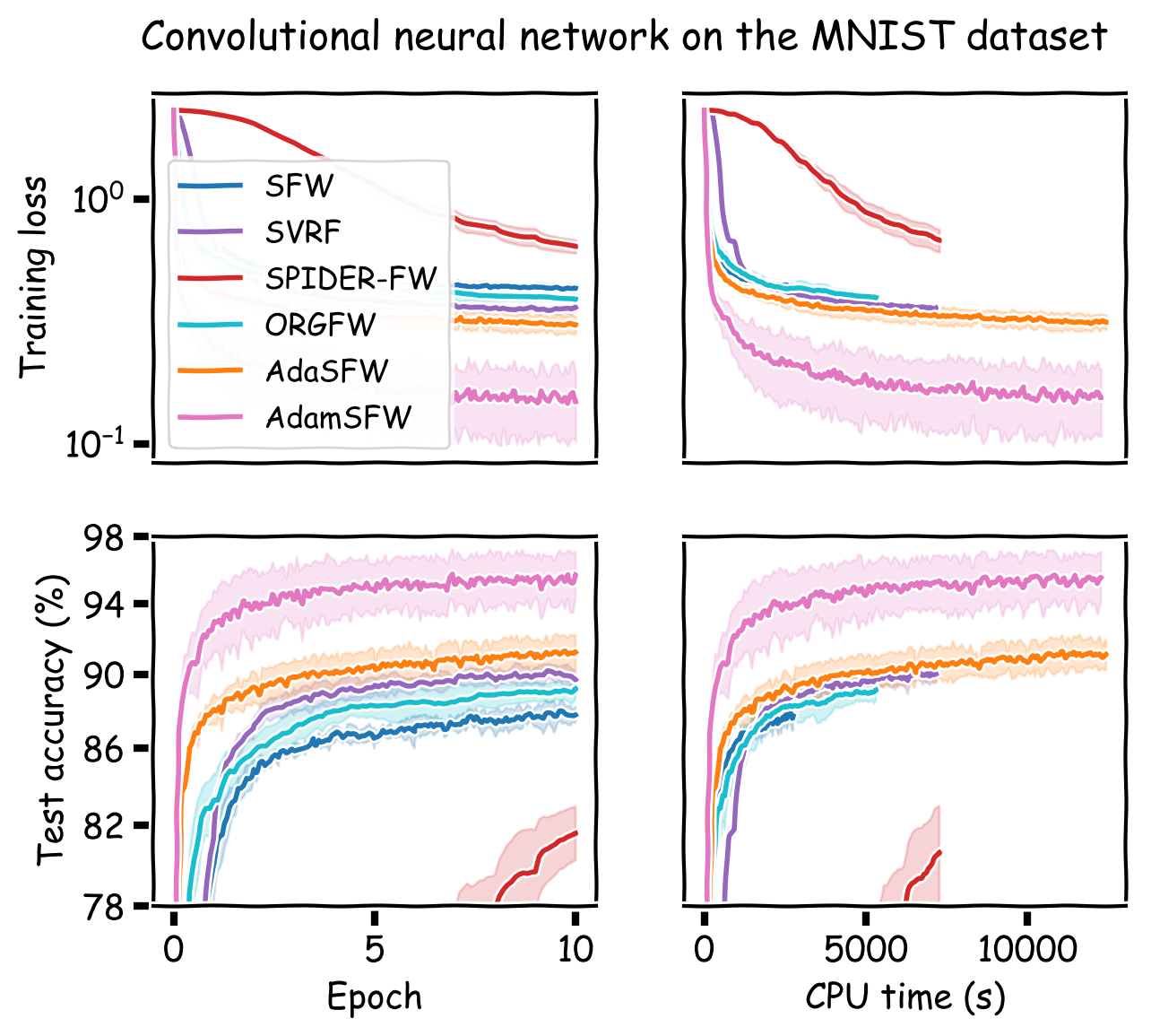
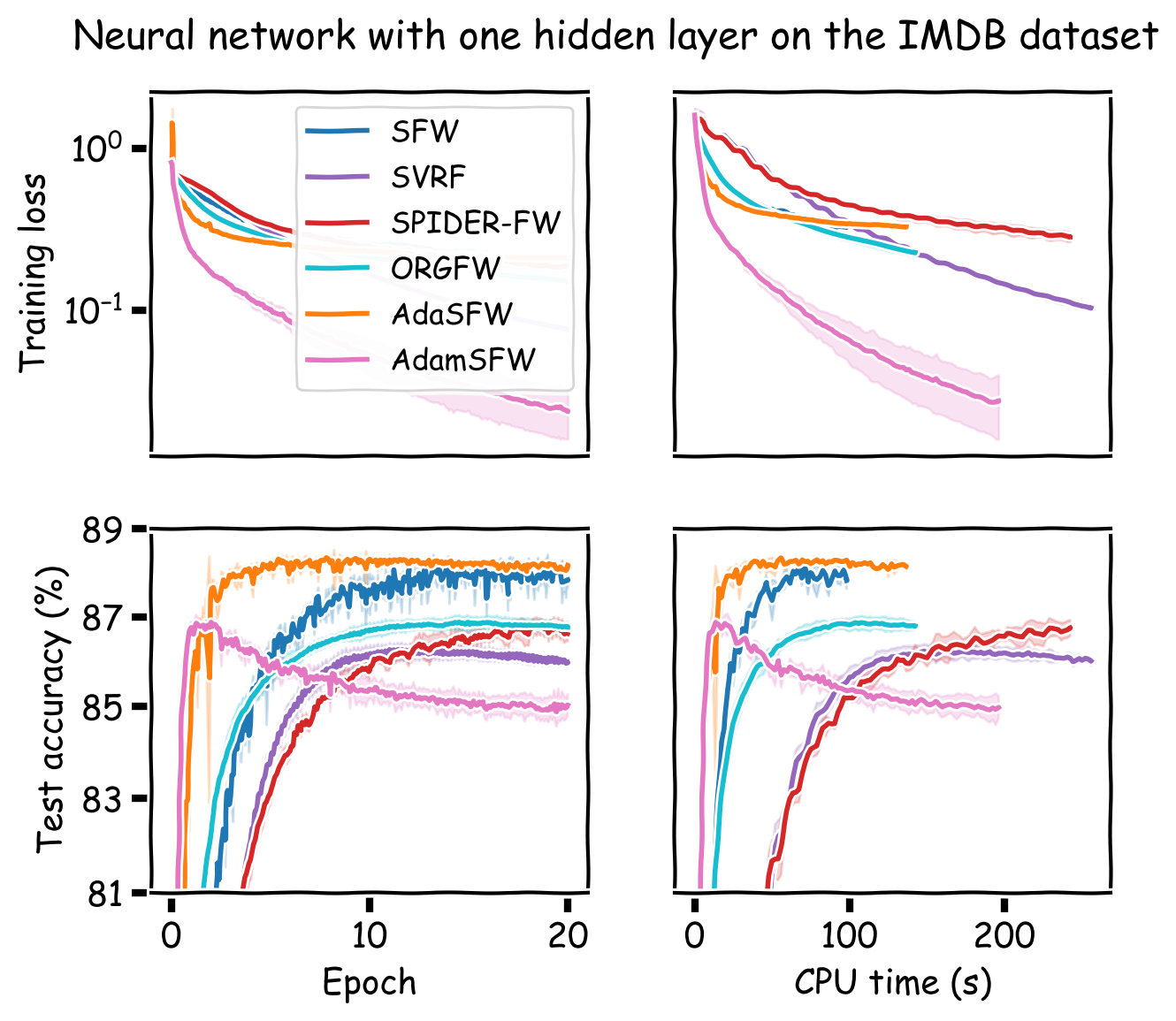
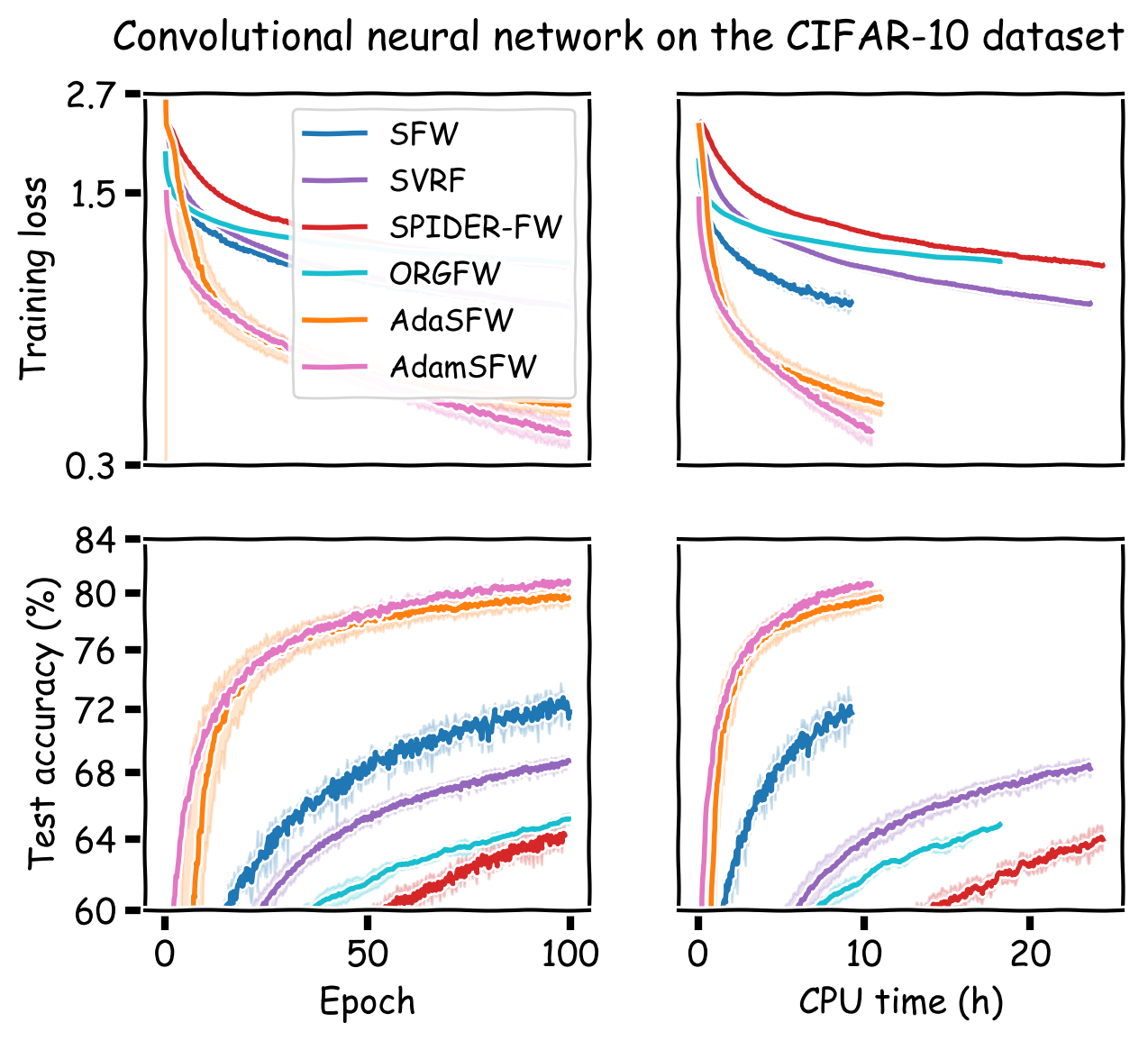
Figure 1. Computational experiments on convex and nonconvex objectives.
References
A. Defazio and L. Bottou. On the ineffectiveness of variance reduced optimization for deep learning. In Advances in Neural Information Processing Systems 32, pages 1755–1765. 2019.
J. C. Duchi, E. Hazan, and Y. Singer. Adaptive subgradient methods for online learning and stochastic optimization. Journal of Machine Learning Research, 12(61):2121–2159, 2011.
M. Frank and P. Wolfe. An algorithm for quadratic programming. Naval Research Logistics Quarterly, 3(1-2):95–110, 1956.
E. Hazan and H. Luo. Variance-reduced and projection-free stochastic optimization. In Proceedings of the 33rd International Conference on Machine Learning, pages 1263–1271, 2016.
G. Lan and Y. Zhou. Conditional gradient sliding for convex optimization. SIAM Journal on Optimization, 26(2):1379–1409, 2016.
E. S. Levitin and B. T. Polyak. Constrained minimization methods. USSR Computational Mathematics and Mathematical Physics, 6(5):1–50, 1966.
H. B. McMahan and M. Streeter. Adaptive bound optimization for online convex optimization. In Proceedings of the 23rd Annual Conference on Learning Theory, 2010.
G. Négiar, G. Dresdner, A. Y.-T. Tsai, L. El Ghaoui, F. Locatello, R. M. Freund, and F. Pedregosa. Stochastic Frank-Wolfe for constrained finite-sum minimization. In Proceedings of the 37th International Conference on Machine Learning. 2020. To appear.
B. T. Polyak. Introduction to Optimization. Optimization Software, 1987.
S. J. Reddi, S. Kale, and S. Kumar. On the convergence of Adam and beyond. In Proceedings of the 6th International Conference on Learning Representations, 2018.
Z. Shen, C. Fang, P. Zhao, J. Huang, and H. Qian. Complexities in projection-free stochastic non-convex minimization. In Proceedings of the 22nd International Conference on Artificial Intelligence and Statistics, pages 2868–2876, 2019.
J. Xie, Z. Shen, C. Zhang, H. Qian, and B. Wang. Efficient projection-free online methods with stochastic recursive gradient. In Proceedings of the 34th AAAI Conference on Artificial Intelligence, pages 6446–6453, 2020.
A. Yurtsever, S. Sra, and V. Cevher. Conditional gradient methods via stochastic path-integrated differential estimator. In Proceedings of the 36th International Conference on Machine Learning, pages 7282–7291. 2019.
Comments