DNN Training with Frank–Wolfe
TL;DR: This is an informal discussion of our recent paper Deep Neural Network Training with Frank–Wolfe by Sebastian Pokutta, Christoph Spiegel, and Max Zimmer, where we study the general efficacy of using Frank–Wolfe methods for the training of Deep Neural Networks with constrained parameters. Summarizing the results, we (1) show the general feasibility of this markedly different approach for first-order based training of Neural Networks, (2) demonstrate that the particular choice of constraints can have a drastic impact on the learned representation, and (3) show that through appropriate constraints one can achieve performance exceeding that of unconstrained stochastic Gradient Descent, matching state-of-the-art results relying on $L^2$-regularization.
Written by Christoph Spiegel.
Motivation
Despite its simplicity, stochastic Gradient Descent (SGD) is still the method of choice for training Neural Networks. Assuming the network is parameterized by some unconstrained weights $\theta$, the standard SGD update can simply be stated as
\[\theta_{t+1} = \theta_t - \alpha \tilde{\,\nabla} L(\theta_t),\]for some given loss function $L$, its $t$-th batch gradient $\tilde{\,\nabla} L(\theta_t)$ and some learning rate $\alpha$. In practice, one of the more significant contributions to this approach for obtaining state-of-the-art performance has come in the form of adding an $L^2$-regularization term to the loss function. Motivated by this, we explored the efficacy of constraining the parameter space of Neural Networks to a suitable compact convex region ${\mathcal C}$. Standard SGD would require a projection step during each update to maintain the feasibility of the parameters in this constrained setting, that is the update would be
\[\theta_{t+1} = \Pi_{\mathcal C} \big( \theta_t - \alpha \tilde{\,\nabla} L(\theta_t) \big),\]where the projection function $\Pi_{\mathcal C}$ maps the input to its closest neighbor in ${\mathcal C}$. Depending on the particular feasible region, such a projection step can be very costly, so we instead explored a more appropriate alternative in the form of the (stochastic) Frank–Wolfe algorithm (SFW) [FW, LP]. Rather than relying on a projection step, SFW calls a linear minimization oracle (LMO) to determine
\[v_t = \textrm{argmin}_{v \in \mathcal C} \langle \tilde{\,\nabla} L(\theta_t), v \rangle,\]and move in the direction of $v_t$ through the update
\[\theta_{t+1} = \theta_t + \alpha ( v_t - \theta_t)\]where $\alpha \in [0,1]$. Feasibility is maintained since the update step takes the convex combination of two points in the convex feasible region. For a more in-depth look at Frank–Wolfe methods check out the Frank-Wolfe and Conditional Gradients Cheat Sheet. In the remainder of this post we will present some of the key findings from the paper.
How to regularize Neural Networks through constraints
We have focused on the case of uniformly applying the same type of constraint, such as a bound on the $L^p$-norm, separately on the weight and bias parameters of each individual layer of the network to achieve a regularizing effect, varying only the diameter of that region. Let us consider some particular types of constraints.
$L^2$-norm ball. Constraining the $L^2$-norm of weights and optimizing them using SFW is most comparable, both in theory and in practice, to SGD with weight decay. The output of the LMO is given by
\[\textrm{argmin}_{v \in \mathcal{B}_2(\tau)} \langle v,x \rangle = -\tau \, x / \|x\|_2,\]that is, it is parallel to the gradient and so, as long as the current iterate of the weights is not close to the boundary of the $L^2$-norm ball, the update of the SFW algorithm is similar to that of SGD given an appropriate learning rate.
Hypercube. Requiring each individual weight of a network or a layer to lie within a certain range, say in $[-\tau,\tau],$ is possibly an even more natural type of constraint. Here the update step taken by SFW however differs drastically from that taken by projected SGD: in the output of the LMO each parameter receives a value of equal magnitude, since
\[\textrm{argmin}_{v \in \mathcal{B}_\infty(\tau)} \langle v,x \rangle = -\tau \, \textrm{sgn}(x),\]so to a degree all parameters are forced to receive a non-trivial update each step.
$L^1$-norm ball and $K$-sparse polytopes. On the other end of the spectrum from the dense updates forced by the LMO of the hypercube are feasible regions whose LMOs return very sparse vectors. When for example constraining the $L^1$-norm of weights of a layer, the output of the LMO is given by the vector with a single non-zero entry equal to $-\tau \, \textrm{sign}(x)$ at a point where $|x|$ takes its maximum. As a consequence, only a single weight, that from which the most gain can be derived, will in fact increase in absolute value during the update step of the Frank–Wolfe algorithm while all other weights will decay and move towards zero. The $K$-sparse polytope of radius $\tau > 0$ is obtained as the intersection of the $L^1$-ball of radius $\tau K$ and the hypercube of radius $\tau$ and generalizes that principle by increasing the absolute value of the $K$ most important weights.
The impact of constraints on learned features
Let us illustrate the impact that the choice of constraints has on the learned representations through a simple classifier trained on the MNIST dataset. The particular network chosen here, for the sake of exposition, has no hidden layers and no bias terms and the flattened input layer of size 784 is fully connected to the output layer of size 10. The weights of the network are therefore represented by a single 784 × 10 matrix, where each of the ten columns corresponds to the weights learned to recognize the ten digits 0 to 9. In Figure 1 we present a visualization of this network trained on the dataset with different types of constraints placed on the parameters. Each image interprets one of the columns of the weight matrix as an image of size 28 × 28 where red represents negative weights and green represents positive weights for a given pixel. We see that the choice of feasible region, and in particular the LMO associated with it, can have a drastic impact on the representations learned by the network when using the stochastic Frank–Wolfe algorithm. For completeness sake we have included several commonly used adaptive variants of SGD in the comparison.
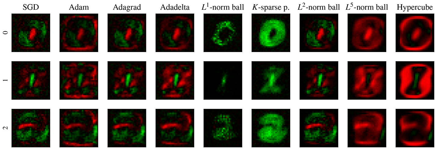
Figure 1. Visualization of the weights in a fully connected no-hidden-layer classifier trained on the MNIST dataset corresponding to the digits 0, 1 and 2. Red corresponds to negative and green to positive weights.
Further demonstrating the impact of constraints on the learned representations, we consider the sparsity of the weights of trained networks. Let the parameter of a network be inactive if its absolute value is smaller than that of its random initialization. To study the effect of constraining the parameters, we trained two different types of networks, a fully connected network with two hidden layers with a total of 26 506 parameters and a convolutional network with 93 322, on the MNIST dataset. In Figure 2 we see that regions spanned by sparse vectors, such as $K$-sparse polytopes, result in noticeably fewer active parameters in the network over the course of training, whereas regions whose LMO forces larger updates in each parameter, such as the Hypercube, result in more active weights.
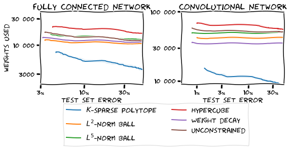
Figure 2. Number of active parameters in two different networks trained on the MNIST dataset.
Achieving state-of-the-art results
Finally, we demonstrate the feasibility of training even very deep Neural Networks using SFW. We trained several state-of-the-art Neural Networks on the CIFAR-10, CIFAR-100, and ImageNet datasets. In Table 1 we show the top-1 test accuracy attained by networks based on the DenseNet, WideResNet, GoogLeNet and ResNeXt architecture on the test sets of these datasets. Here we compare networks with unconstrained parameters trained using SGD with momentum both with and without weight decay as well as networks whose parameters are constrained in their $L^2$-norm or $L^\infty$-norm and which were trained using SFW with momentum added. We can observe that, when constraining the $L^2$-norm of the parameters, SFW attains performance exceeding that of standard SGD and matching the state-of-the-art performance of SGD with weight decay. When constraining the $L^\infty$-norm of the parameters, SFW does not quite achieve the same performance as SGD with weight decay, but a regularization effect through the constraints is nevertheless clearly present, as it still exceeds the performance of SGD without weight decay. We furthermore note that, due to the nature of the LMOs associated with these particular regions, runtimes were comparable.
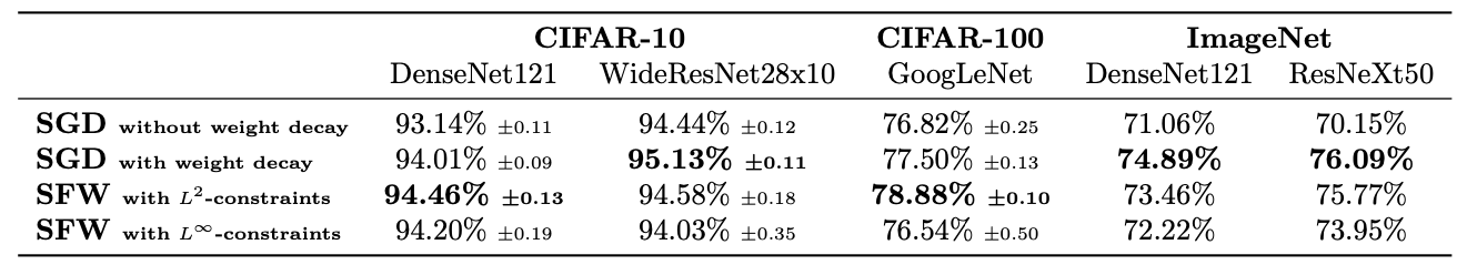
Table 1. Test accuracy attained by several deep Neural Networks trained on the CIFAR-10, CIFAR-100, and ImageNet datasets. Parameters trained with SGD were unconstrained.
Reproducibility
We have made our implementations of the various stochastic Frank–Wolfe methods considered in the paper available online both for PyTorch and for TensorFlow under github.com/ZIB-IOL/StochasticFrankWolfe. There you will also find a list of Google Colab notebooks that allow you to recreate all the experimental results presented here.
References
[FW] Frank, M., & Wolfe, P. (1956). An algorithm for quadratic programming. Naval research logistics quarterly, 3(1‐2), 95-110. pdf
[LP] Levitin, E. S., & Polyak, B. T. (1966). Constrained minimization methods. Zhurnal Vychislitel’noi Matematiki i Matematicheskoi Fiziki, 6(5), 787-823. pdf
Comments