Linear Bandits on Uniformly Convex Sets
TL;DR: This is an informal summary of our recent paper Linear Bandit on Uniformly Convex Sets by Thomas Kerdreux, Christophe Roux, Alexandre d’Aspremont, and Sebastian Pokutta. We show that the strong convexity of the action set $\mathcal{K}\subset\mathbb{R}^n$ in the context of linear bandits leads to a gain of a factor of $\sqrt{n}$ in the pseudo-regret bounds. This improvement was previously known in only two settings: when $\mathcal{K}$ is the simplex or an $\ell_p$ ball with $p\in]1,2]$ [BCY]. When the action set is $q$-uniformly convex (with $q\geq 2$) but not necessarily strongly convex, we obtain pseudo-regret bounds of the form $\mathcal{O}(n^{1/q}T^{1/p})$ (with $1/p+1/q=1$), i.e., with a dimension dependency smaller than $\sqrt{n}$.
Written by Thomas Kerdreux.
In this post, we continue our journey toward analyzing Machine Learning algorithms according to the constraint sets’ (in the context of optimization) or action sets’ (in the context of online learning or bandits) structural properties. In our recent paper [KDPa], we focused on the case of projection-free optimization and proved accelerated convergence rates when the set is (locally or globally) uniformly convex. This allowed us to understand better how to manipulate such structures and come up with local set assumptions. We detail these structural assumptions in [KDPb] and provide other connections between the uniform convexity of the set and problems in Machine Learning, e.g., with generalization bounds. Here we focus on the linear bandit setting. We design and analyze algorithms that are not projection-free. Let us now first recall the linear bandit setting.
Linear Bandits
Linear Bandit Setting
Input: Consider a compact convex action set $\mathcal{K}\subset\mathbb{R}^n$.
For $t=0, 1, \ldots, T $ do:
$\qquad$ Nature decides on a loss vector $c_t\in\mathcal{K}^\circ$.
$\qquad$ The bandit algorithm picks an action $a_t\in\mathcal{K}$.
$\qquad$ The bandit observes the cost $\langle c_t; a_t\rangle$ of its action but not $c_t$.
The goal of the bandit algorithm is to incur the smallest cumulative cost $\sum_{t=1}^{T}\langle c_t; a_t\rangle$. The bandit framework is also known as the partial-information setting (as opposed to full-information setting which is online learning) because the algorithm does not have access to the entire $c_t$ to update its strategy. The performance of a bandit algorithm is then measured via the regret $R_T$,
\[\tag{Regret} R_T = \sum_{t=1}^{T} \langle c_t; a_t\rangle - \underset{a\in\mathcal{K}}{\text{min }} \sum_{t=1}^{T} \langle c_t; a_t\rangle,\]where the second term represents the cost of playing the single best action in hindsight. Theoretical upper bounds on the regret $R_T$ then serve as a designing criterion of bandit algorithms. Since bandit algorithms all employ internal randomization procedures, we consider expected or high-probability regret bounds with respect to this internal randomness. However, these types of bounds remain challenging to obtain, and pseudo-regret bounds are often considered as a important first step. Denote by $\mathbb{E}$ the expectation with respect to the bandit randomness, the pseudo-regret $\bar{R}_T$ is defined as
\[\tag{Pseudo-Regret} \bar{R}_T = \mathbb{E}\Big(\sum_{t=1}^{T}\langle c_t; a_t\rangle\Big) - \underset{a\in\mathcal{K}}{\text{min }} \mathbb{E}\Big(\sum_{t=1}^{T} \langle c_t; a_t\rangle\Big).\]In the linear bandit setting, the algorithm can solely leverage the structure of the constraint set to achieve accelerated regret bounds. Indeed, the loss is linear so that there is no functional lower-curvature assumption, e.g., no strong convexity. For a general compact convex set the pseudo-regret bound is of $\tilde{\mathcal{O}}(n\sqrt{T})$ and we are aware of better pseudo-regret bounds of $\tilde{\mathcal{O}}(\sqrt{nT})$ only when the action set $\mathcal{K}$ is a simplex or an $\ell_p$ ball with $p\in]1,2]$ [BCB,BCY]. Is there a more general mechanism that explain the accelerated regret bounds with the $\ell_p$ balls? What happens with $p>2$?
Preliminaries
We need to introduce a few simple notions of functional analysis and convex geometry. Although we do not enter the proof’s technical details in this post, we try to convey the core ingredient on which the proof relies. For $p\in]1,2]$, a convex differentiable function $f$ is $(L, p)$-Hölder smooth on $\mathcal{K}$ with respect to a norm $\norm{\cdot}$ if and only if for any $(x,y)\in\mathcal{K}\times\mathcal{K}$
\[\tag{Hölder-Smoothness} f(y) \leq f(x) + \langle \nabla f(x); y-x \rangle + \frac{L}{p} \norm{y-x}^p.\]It generalizes the classical notion of $L$-smoothness of the function. This assumption will play a role because it is dual to uniform convexity, i.e., when a function is strongly convex then its Fenchel conjugate is smooth. The Bregman divergence of $F: \mathcal{D}\rightarrow\mathbb{R}$ is defined for $(x,y)\in\bar{\mathcal{D}}\times\mathcal{D}$ by
\[\tag{Bregman-Divergence} D_F(x,y) = F(x) - F(y) - \langle x-y ; \nabla F(y)\rangle.\]The key of our pseudo-regret upper-bounds analysis is to relate the set’s uniform convexity with the Hölder smoothness of a function related to $\mathcal{K}$. This then allows us to upper bound a Bregman Divergence that naturally arises in the computations.
Before going on with introducing the uniform convexity properties of the set, let us first explain the requirement that $c\in\mathcal{K}^\circ$. We write $\mathcal{K}^\circ$ for the polar of $\mathcal{K}$ and it is defined as follows
\[\tag{Polar} \mathcal{K}^\circ := \big\{ c\in\mathbb{R}^n ~|~ \langle c; a\rangle \leq 1~\forall a\in\mathcal{K} \big\}.\]In other words, constraining Nature to pick a loss vector $c\in\mathcal{K}^\circ$ ensures that whatever the action $a\in\mathcal{K}$ taken by the bandit, it will incur a bounded loss $\langle c; a\rangle\leq 1$.
Finally, both the algorithm and the analysis of our pseudo-regret bounds rely on the notion of gauge, which is essentially an extension of a norm. For a compact convex set $\mathcal{K}$ , the gauge $\norm{\cdot}_{\mathcal{K}}$ of $\mathcal{K}$ is defined at $x\in\mathbb{R}^n$ as
\[\tag{Gauge of $\mathcal{K}$} \|x\|_\mathcal{K} := \text{inf}\{\lambda>0~|~ x\in\lambda\mathcal{K}\}.\]When $\mathcal{K}$ is centrally symmetric and contains $0$ in its interior, then the gauge of $\mathcal{K}$ is a norm and $\mathcal{K}$ is the unit ball of its norm (indeed $\norm{x}_\mathcal{K} \leq 1 \Leftrightarrow x\in\mathcal{K}$). The gauge function is hence a natural way to associate a function to a set.
Action Set Assumptions
A closed set $\mathcal{C}\subset\mathbb{R}^d$ is $(\alpha, q)$-uniformly convex with respect to a norm $\norm{\cdot}$, if for any $x,y \in \mathcal{C}$, any $\eta\in[0,1]$ and any $z\in\mathbb{R}^d$ with $\norm{z} = 1$, we have
\[\tag{Uniform Convexity} \eta x + (1-\eta) y + \eta (1 - \eta ) \alpha \norm{x-y}^q z \in \mathcal{C}.\]At a high level, this property is a global quantification of the set curvature that subsumes strong convexity. In finite-dimensional spaces, the $\ell_p$ balls are a fundamental example. For $p\in ]1,2]$, the $\ell_p$ balls are strongly convex (or $(\alpha,2)$-uniformly convex) and $p$-uniformly convex (but not strongly convex) for $p>2$. $p$-Schatten norms with $p>1$ or various group norms are also typical examples.
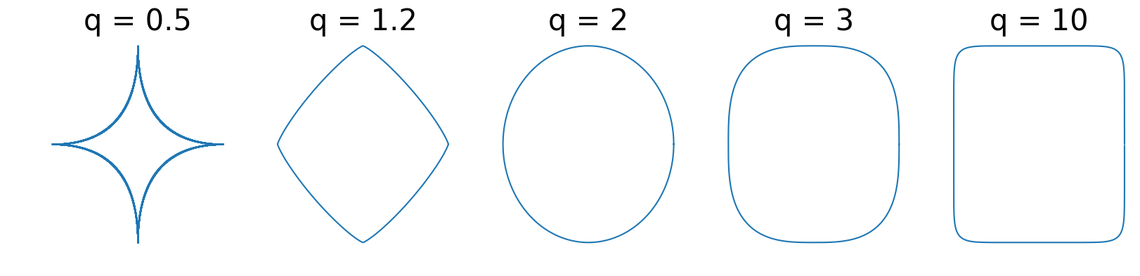
Figure 1. Examples of $\ell_q$ balls.
As outlined in [KDPa,KDPb], scaling inequalities offer an interesting equivalent definition of $(\alpha,q)$-uniform convexity. Namely, $\mathcal{K}$ is $(\alpha, q)$-uniformly convex with respect to $\norm{\cdot}$ if and only if for any $x\in\partial\mathcal{K}$, \(c \in N_{\mathcal{K}}(x) := \big\{c\in\mathbb{R}^n \mid \langle c; x-y\rangle \geq 0 \ \forall y\in\mathcal{K}\big\}\) (the normal cone) and $y\in\mathcal{K}$, we have
\[\tag{Scaling Inequality} \langle c; x- y\rangle \geq \alpha \|c\|_\star \|x-y\|^q.\]A natural question arises when using this less considered (as opposed to the case for function) notion of uniform convexity for sets: does the uniform convexity of the set translate into a uniform convexity property of the gauge function?
It does and the result is quite classical. We survey such results in [KDPb]. Let us recall it here:
\[\mathcal{K} \text{ is } (\alpha, q)\text{-uniformly convex} \Leftrightarrow \norm{\cdot}^q_{\mathcal{K}} \text{ is } (\alpha^\prime, q)\text{-uniformly convex for some } \alpha^\prime>0.\]Note also that the choice to constrain the loss vector $c_t\in\mathcal{K}^\circ$ now allows us to easily manipulate the gauge function and its dual. Indeed, we have that \(\norm{\cdot}_{\mathcal{K}}^\star = \norm{\cdot}_{\mathcal{K}^\circ}\). We can then also manipulate the Fenchel conjugate function (beware, however, that dual norm and Fenchel conjugate of the norm are not equal) of \(\norm{\cdot}^q_{\mathcal{K}}\) to link it with a power of \(\norm{\cdot}_{\mathcal{K}^\circ}\). Without entering into technical details, the high-level idea is that the uniform convexity of $\mathcal{K}$ ensures the uniform convexity of a power of the gauge function of \(\norm{\cdot}_{\mathcal{K}}\) and ultimately the Hölder Smoothness of the Fenchel conjugate of a power of the gauge function of \(\norm{\cdot}_{\mathcal{K}^\circ}\).
Bandit Algorithm on Uniformly Convex Sets and Pseudo-Regret Bounds
Similarly to [BCB,BCY] we apply a bandit version of Online Stochastic Mirror Descent. The sole difference is that we consider specific barrier $F_{\mathcal{K}}$ function for uniformly convex action set $\mathcal{K}$ and we account for the reference radius, i.e., the $r>0$ such that $\ell_1(r)\subset\mathcal{K} $. For $x\in\text{Int}(\mathcal{K})$ the barrier function is defined as follows
\[\tag{Barrier Function} F_{\mathcal{K}}(x) := - \ln(1-\norm{x}_{\mathcal{K}}) - \norm{x}_{\mathcal{K}}.\]Here, we do not detail the action’s sampling scheme; see the details in [KCDP]. Note that the algorithm is adaptive because it does not require knowledge of the parameter of uniform convexity.
Algorithm 1: Linear Bandit Mirror Descent
Input: $\eta>0$, $\gamma\in]0,1[$, $\mathcal{K}$ smooth and strictly convex such that \(\ell_1(r)\subset\mathcal{K}\).
Initialize: \(x_1\in\text{argmin}_{x\in(1-\gamma)\mathcal{K}}F_{\mathcal{K}}(x)\)
For $t=1, \ldots, T$ do:
$\qquad$ Sample $a_t\in\mathcal{K}$ $\qquad \vartriangleright$ Bandit internal randomization.
$\qquad$ \(\tilde{c}_t \gets \frac{n}{r^2} (1-\xi_t) \frac{\langle a_t; c_t\rangle }{1-\norm{x_t}_{\mathcal{K}}}a_t\) $\qquad \vartriangleright$ Estimate loss vector
$\qquad$ \(x_{t+1} \gets \underset{y\in(1-\gamma)\mathcal{K}}{\text{argmin }} D_{F_{\mathcal{K}}}\big(y, \nabla F_{\mathcal{K}}^*(\nabla F_{\mathcal{K}}(x_t)- \eta \tilde{c}_t)\big) \big)\) $\qquad \vartriangleright$ Mirror Descent step
We now cite our analysis of the pseudo-regret bounds on Algorithm 1 when the set $\mathcal{K}$ is strongly convex.
Theorem 1: Linear Bandit on Strongly Convex Set
Consider a compact convex set $\mathcal{K}$ that is centrally symmetric with non-empty interior. Assume $\mathcal{K}$ is smooth and $\alpha$-strongly convex set with respect to \(\norm{\cdot}_{\mathcal{K}}\) and \(\ell_2(r)\subset \mathcal{K} \subset \ell_{\infty}(R)\) for some \(r,R>0\).
Consider running Algorithm 1 with the barrier function \(F_{\mathcal{K}}(x)=-\ln\big(1-\norm{x}_{\mathcal{K}}\big) - \norm{x}_{\mathcal{K}}\), and \(\eta=\frac{1}{\sqrt{nT}}\), \(\gamma=\frac{1}{\sqrt{T}}\). Then, for \(T\geq 4n\big(\frac{R}{r}\big)^2\) we have
\[
\bar{R}_T \leq \sqrt{T} + \sqrt{nT}\ln(T)/2 + L\sqrt{nT} = \tilde{\mathcal{O}}(\sqrt{nT}),
\]
where $L=(R/r)^2(5\alpha + 4)/\alpha$.
In this blog, we do not detail the technical proof. The core idea is to leverage the strong convexity of \(\mathcal{K}\) by noting that it implies the smoothness of \(\frac{1}{2}\norm{\cdot}_{\mathcal{K}^\circ}^2\) on $\mathcal{K}$. It then provides an upper bound on the Bregman Divergence of \(\frac{1}{2}\norm{\cdot}_{\mathcal{K}^\circ}^2\). It is a crucial term that emerges when we carefully factorized the terms in the upper bound on the progress of a Mirror Descent step in Algorithm 1. We hence obtain pseudo-regret bounds in \(\tilde{\mathcal{O}}(\sqrt{nT})\) for a generic family of sets. Such accelerated pseudo-regret bounds were previously known only in the case of the simplex or the $\ell_p$ ball with $p\in]1,2]$.
We obtain a more generic version when the action set is $(\alpha,q)$-uniformly convex with $q \geq 2$.
Theorem 2: Linear Bandit on Uniformly Convex Set
Let $\alpha>0$, $q\geq 2$, and $p\in]1,2]$ such that $1/p + 1/q=1$ and consider a compact convex set $\mathcal{K}$ that is centrally symmetric with non-empty interior. Assume $\mathcal{K}$ is smooth and $(\alpha, q)$-uniformly convex set with respect to \(\norm{\cdot}_{\mathcal{K}}\) and \(\ell_q(r)\subset \mathcal{K} \subset \ell_{\infty}(R)\) for some $r,R>0$. Consider running Algorithm A with the barrier function \(F_{\mathcal{K}}(x)=-\ln\big(1-\norm{x}_{\mathcal{K}}\big) - \norm{x}_{\mathcal{K}}\), and $\eta=1/(n^{1/q}T^{1/p})$, $\gamma=1/\sqrt{T}$. Then for $T\geq 2^p n \big(\frac{R}{r}\big)^p$ we have
\[
\bar{R}_T \leq \sqrt{T} + n^{1/q} T^{1/p} \ln(T)/2 + ((1/2)^{2-p} + L) \Big(\frac{R}{r}\Big)^p n^{1/q} T^{1/p} = \tilde{\mathcal{O}}(n^{1/q} T^{1/p}),
\]
where $L=2p(1 + (q/(2\alpha))^{1/(q-1)})$.
Here, the rate with uniformly convex set is not an interpolation between the $\tilde{\mathcal{O}}(\sqrt{nT})$ of strongly convex sets and the $\tilde{\mathcal{O}}(n\sqrt{T})$ when the set is compact convex. Another trade-off appears. Indeed, the pseudo-regret bounds dimension-dependence can be arbitrarily smaller than $\sqrt{n}$ while the rate in terms of iteration can get arbitrarily close to $\mathcal{O}(T)$.
Conclusion
When the action set is strongly convex, we design a barrier function leading to a bandit algorithm with pseudo-regret in $\tilde{\mathcal{O}}(\sqrt{nT})$. We hence drastically extend the family of action sets for which such pseudo-regret holds, answering an open question of [BCB]. To our knowledge, a $\tilde{\mathcal{O}}(\sqrt{nT})$ bound was known only when the action set is a simplex or an $\ell_p$ ball with $p\in]1,2]$.
When the set is $(\alpha, q)$-uniformly convex with $q\geq 2$, we assume in Theorem 1 and 2 that $\ell_q(r)$ is contained in the action set $\mathcal{K}$. It is restrictive but allows us to first prove improved pseudo-regret bounds outside the explicit $\ell_p$ case. Removing this assumption is an interesting research direction. However, it is not clear that the current classical algorithmic scheme with a barrier function is best adapted to leverage the strong convexity of the action set. Indeed, in the case of online linear learning, [HLGS] show that the simple FTL allows obtaining accelerated regret bounds.
At a high level, this work is an example of the favorable dimension-dependency of the sets’ uniform convexity assumptions for the pseudo-regret bounds. It is crucial for large-scale machine learning. Besides, the uniform convexity structures for the sets are much less developed and understood than their functional counterpart, see, e.g., [KDPb]. Arguably, this stems from a tendency in machine learning to consider the constraints to be theoretically interchangeable with penalization. It is often not quite accurate in terms of convergence results, and the algorithmic strategies developed differ. The linear bandit setting is a simple example where such symmetry is structurally not relevant.
References
[BCB] Bubeck, Sébastian, Cesa-Bianchi, Nicolo. “Regret Analysis of Stochastic and Nonstochastic Multi-armed Bandit Problems”. Foundations & Trends in Machine Learning. 2012. pdf
[BCY] Bubeck, Sébastien, Michael Cohen, and Yuanzhi Li. “Sparsity, variance and curvature in multi-armed bandits.” Algorithmic Learning Theory. PMLR, 2018. pdf
[HLGS] Huang, R., Lattimore, T., György, A., and Szepesvári, C. “Following the leader and fast rates in online linear prediction: Curved constraint sets and other regularities”. The Journal of Machine Learning Research, 18(1), 2017. pdf
[KCDP] Kerdreux, Thomas, Christophe Roux, Alexandre d’Aspremont, and Sebastian Pokutta. “Linear Bandit on uniformly convex sets.” pdf
[KDPa] Kerdreux, Thomas, Alexandre d’Aspremont, and Sebastian Pokutta. “Projection-free optimization on uniformly convex sets.” AISTATS. 2021. pdf
[KDPb] Kerdreux, Thomas, Alexandre d’Aspremont, and Sebastian Pokutta. “Local and Global Uniform Convexity Conditions.” 2021. pdf
Comments