FrankWolfe.jl: A high-performance and flexible toolbox for Conditional Gradients
TL;DR: We present $\texttt{FrankWolfe.jl}$, an open-source implementation in Julia of several popular Frank-Wolfe and Conditional Gradients variants for first-order constrained optimization. The package is designed with flexibility and high-performance in mind, allowing for easy extension and relying on few assumptions regarding the user-provided functions. It supports Julia’s unique multiple dispatch feature, and interfaces smoothly with generic linear optimization formulations using $\texttt{MathOptInterface.jl}$.
Written by Alejandro Carderera and Mathieu Besançon.
What does the package do?
The $\texttt{FrankWolfe.jl}$ Julia package aims at solving problems of the form: \(\tag{minProblem} \begin{align} \label{eq:minimizationProblem} \min\limits_{\mathbf{x} \in \mathcal{C}} f(\mathbf{x}), \end{align}\) where $\mathcal{C} \subseteq \mathbb{R}^d$ is a convex compact set and $f(\mathbf{x})$ is a differentiable function, through the use of Frank-Wolfe [FW] (also known as Conditional Gradient [LP]) algorithm variants. The two main ingredients that the package uses to solve this problem are:
- A First-Order Oracle (FOO): Given $\mathbf{x} \in \mathcal{C}$, the oracle returns $\nabla f(\mathbf{x})$.
- A Linear Minimization Oracle (LMO): Given $\mathbf{x}\in \mathbb{R}^d$, the oracle returns $\mathbf{v} \in \operatorname{argmin}_{\mathbf{x} \in \mathcal{C}} \langle \mathbf{d}, \mathbf{x}\rangle$.
This bypasses the need to use projection oracles onto $\mathcal{C}$, which can be extremely advantageous as solving an LP over $\mathcal{C}$ can be much cheaper than solving a quadratic (projection) problem over the same set. Such is the case for the nuclear norm ball, as solving an LP over this convex set simply requires computing the left and right singular vectors associated with the largest singular value, whereas projecting onto this feasible region requires computing a full SVD decomposition. See [CP] for more examples and for more background information on the package see also our software overview of the package [BCP].
How do I get started
In a Julia session, type ] to switch to package mode:
julia> ]
(@v1.6) pkg>
See the Julia documentation
for more examples and advanced usage of the package manager.
You can then add the package with the add command:
(@v1.6) pkg> add https://github.com/ZIB-IOL/FrankWolfe.jl
Soon it will also be directly available through the package manager.
And why should you care?
Although the Frank-Wolfe algorithm and its variants have been studied for more than half a decade and have gained a lot of attention due to their favorable theoretical and computational properties, no de-facto implementation exists. The goal of the package is to become a reference open-source implementation for practitioners in need of a flexible and efficient first-order method and for researchers developing and comparing new approaches on similar classes of problems.
Algorithm variants included in the package
We summarize below the central ideas of the variants implemented in the package and highlight in Table 1 key properties that can drive the choice of a variant on a given use case. More information about the variants can be found in the references provided. We mention briefly that most variants also work for the nonconvex case, providing some locally optimal solution in this case.
Standard Frank-Wolfe. The simplest Frank-Wolfe variant is included in the package. It has the lowest memory requirements out of all the variants, as in its simplest form only requires keeping track of the current iterate. As such it is suited for extremely large problems. However, in certain cases, this comes at the cost of speed of convergence in terms of iteration count, when compared to other variants. As an example, when minimizing a strongly convex and smooth function over a polytope this algorithm might converge sublinearly, whereas the three variants that will be presented next converge linearly.
Away-step Frank-Wolfe. One of the most popular Frank-Wolfe variants is the Away-step Frank-Wolfe (AFW) algorithm [GM, LJ]. While the standard FW algorithm can only move towards extreme points of $\mathcal{C}$, the AFW can move away from some extreme points of $\mathcal{C}$, hence the name of the algorithm. To be more specific, the AFW algorithm moves away from vertices in its active set at iteration $t$, denoted by $\mathcal{S}_t$, which contains the set of vertices $\mathbf{v}_k$ for $k<t$ that allow us to recover the current iterate as a convex combination. This algorithm expands the range of directions that the FW algorithm can move along, at the expense of having to explicitly maintain the current iterate as a convex decomposition of extreme points.
Lazifying Frank-Wolfe variants. One running assumption for the two previous variants is that calling the LMO is cheap. There are many applications where calling the LMO in absolute terms is costly (but is cheap in relative terms when compared to performing a projection). In such cases, one can attempt to lazify FW algorithms, to avoid having to compute $\operatorname{argmin}_{\mathbf{v}\in\mathcal{C}}\left\langle\nabla f(\mathbf{x}_t),\mathbf{v} \right\rangle$ by calling the LMO, settling for solutions that guarantee enough progress [BPZ]. This allows us to substitute the LMO by a Weak Separation Oracle while maintaining essentially the same convergence rates. In practice, these algorithms search for appropriate vertices among the vertices in a cache, or the vertices in the active set $\mathcal{S}_t$, and can be much faster in wall-clock time. In the package, both AFW and FW have lazy variants while the BCG algorithm is lazified by design.
Blended Conditional Gradients. The FW and AFW algorithms, and their lazy variants share one feature: they attempt to make primal progress over a reduced set of vertices. The AFW algorithm does this through away steps (which do not increase the cardinality of the active set), and the lazy variants do this through the use of previously exploited vertices. A third strategy that one can follow is to explicitly blend Frank-Wolfe steps with gradient descent steps over the convex hull of the active set (note that this can be done without requiring a projection oracle over $\mathcal{C}$, thus making the algorithm projection-free). This results in the Blended Conditional Gradient (BCG) algorithm [BPTW], which attempts to make as much progress as possible over the convex hull of the current active set $\mathcal{S}_t$ until it automatically detects that in order to further make further progress it requires additional calls to the LMO and new atoms.
Stochastic Frank-Wolfe. In many problem instances, evaluating the FOO at a given point is prohibitively expensive. In such cases, one usually has access to a Stochastic First-Order Oracle (SFOO), from which one can build a gradient estimator. This idea, which has powered much of the success of deep learning, can also be applied to the Frank-Wolfe algorithm [HL], resulting in the Stochastic Frank-Wolfe (SFW) algorithm and its variants.
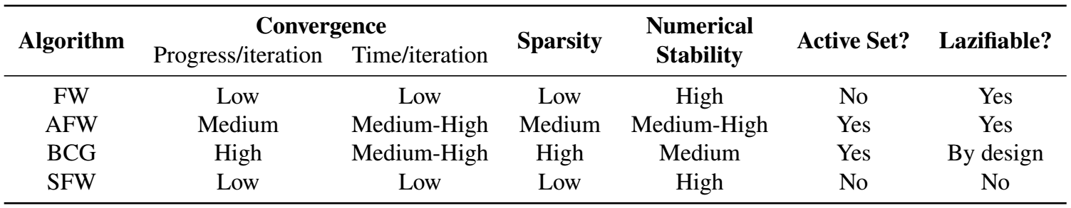
Table 1. Schematic comparison of the different algorithmic variants.
Package design characteristics
Unlike disciplined convex frameworks or algebraic modeling languages such as $\texttt{Convex.jl}$ or $\texttt{JuMP.jl}$, our framework allows for arbitrary Julia functions defined outside of a Domain-Specific Language. Users can provide their gradient implementation or leverage one of the many automatic differentiation packages available in Julia.
One central design principle of $\texttt{FrankWolfe.jl}$ is to rely on few assumptions regarding the user-provided functions, the atoms returned by the LMO, and their implementation. The package works for instance out of the box when the LMO returns Julia subtypes of AbstractArray, representing finite-dimensional vectors, matrices or higher-order arrays.
Another design principle has been to favor in-place operations and reduce memory allocations when possible, since these can become expensive when repeated at all iterations. This is reflected in the memory emphasis mode (the default mode for all algorithms), where as many computations as possible are performed in-place as well as in the gradient interface, where the gradient function is provided with a variable to write into rather than reallocating every time a gradient is computed. The performance difference can be quite pronounced for problems in large dimensions, for example passing a gradient of size 7.5GB on a state-of-the-art machine is about 8 times slower than an in-place update.
Finally, default parameters are chosen to make all algorithms as robust as possible out of the box, while allowing extension and fine tuning for advanced users. For example, the default step size strategy for all (but the stochastic variant) is the adaptive step size rule of [PNAM], which in computations not only usually outperforms both line search and the short step rule by dynamically estimating the Lipschitz constant but also overcomes several issues with the limited additive accuracy of traditional line search rules. Similarly, the BCG variant automatically upgrades the numerical precision for certain subroutines if numerical instabilities are detected.
Linear minimization oracle interface
One key step of FW algorithms is the linear minimization step which, given first-order information at the current iterate, returns an extreme point of the feasible region that minimizes the linear approximation of the function. It is defined in $\texttt{FrankWolfe.jl}$ using a single function:
function compute_extreme_point(lmo::LMO, direction::D; kwargs...)::V
  # ...
end
The first argument $\texttt{lmo}$ represents the linear minimization oracle for the specific problem. It encodes the feasible region $\mathcal{C}$, but also some algorithmic parameters or state. This is especially useful for the lazified FW variants, as in these cases the LMO types can take advantage of caching, by storing the extreme vertices that have been computed in previous iterations and then looking up vertices from the cache before computing a new one.
The package implements LMOs for commonly encountered feasible regions including $L_p$-norm balls, $K$-sparse polytopes, the Birkhoff polytope, and the nuclear norm ball for matrix spaces, leveraging known closed forms of extreme points. The multiple dispatch mechanism allows for different implementations of a single LMO with multiple direction types. The type $\texttt{V}$ used to represent the computed vertex is also specialized to leverage the properties of extreme vertices of the feasible region. For instance, although the Birkhoff polytope is the convex hull of all doubly stochastic matrices of a given dimension, its extreme vertices are permutation matrices that are much sparser in nature. We also leverage sparsity outside of the traditional sense of nonzero entries. When the feasible region is the nuclear norm ball in $\mathbb{R}^{N\times M}$, the vertices are rank-one matrices. Even though these vertices are dense, they can be represented as the outer product of two vectors and thus be stored with $\mathcal{O}(N+M)$ entries instead of $\mathcal{O}(N\times M)$ for the equivalent dense matrix representation. The Julia abstract matrix representation allows the user and the library to interact with these rank-one matrices with the same API as standard dense and sparse matrices.
In some cases, users may want to define a custom feasible region that does not admit a closed-form linear minimization solution. We implement a generic LMO based on $\texttt{MathOptInterface.jl}$, thus allowing users on the one hand to select any off-the-shelf LP, MILP, or conic solver suitable for their problem, and on the other hand to formulate the constraints of the feasible domain using the $\texttt{JuMP.jl}$ or $\texttt{Convex.jl}$ DSL. Furthermore, the interface is naturally extensible by users who can define their own LMO and implement the corresponding $\texttt{compute_extreme_point}$ method.
Numeric type genericity
The package was designed from the start to be generic over both the used numeric types and data structures. Numeric type genericity allows running the algorithms in extended fixed or arbitrary precision, e.g., the package works out-of-the-box with $\texttt{Double64}$ and $\texttt{BigFloat}$ types. Extended precision is essential for high-dimensional problems where the condition number of computed gradients etc., become too high. For some well-conditioned problems, reduced precision is sometimes sufficient to achieve the desired tolerance. Furthermore, it opens the possibility of gradient computation and LMO steps on hardware accelerators such as GPUs.
Examples
We will now present a few examples that highlight specific features of the package. The full code of each example (and several more) can be found in the examples folder of the repository.
Matrix completion
Missing data imputation is a key topic in data science. Given a set of observed entries from a matrix $Y \in \mathbb{R}^{m\times n}$, we want to compute a matrix $X \in \mathbb{R}^{m\times n}$ that minimizes the sum of squared errors on the observed entries. As it stands this problem formulation is not well-defined or useful, as one could minimize the objective function simply by setting the observed entries of $X$ to match those of $Y$, and setting the remaining entries of $X$ arbitrarily. However, this would not result in any meaningful information regarding the unobserved entries in $Y$, which is one of the key tasks in missing data imputation. A common way to solve this problem is to reduce the degrees of freedom of the problem in order to recover the matrix $Y$ from a small subset of its entries, e.g., by assuming that the matrix $Y$ has low rank. Note that even though the matrix $Y$ has $m\times n$ coefficients, if it has rank $r$, it can be expressed using only $(m + n - r)r$ coefficients through its singular value decomposition. Finding the matrix $X \in \mathbb{R}^{m\times n}$ with minimum rank whose observed entries are equal to those of $Y$ is a non-convex problem that is $\exists \mathbb{R}$-hard. A common proxy for rank constraints is the use of constraints on the nuclear norm of a matrix, which is equal to the sum of its singular values, and can model the convex envelope of matrices of a given rank. Using this property, one of the most common ways to tackle matrix completion problems is to solve: \(\begin{align} \min_{\|X\|_{*} \leq \tau} \sum_{(i,j)\in \mathcal{I}} \left( X_{i,j} - Y_{i,j}\right)^2, \label{Prob:matrix_completion} \end{align}\) where $\tau>0$ and $\mathcal{I}$ denotes the indices of the observed entries of $Y$. In this example, we compare the Frank-Wolfe implementation from the package with a Projected Gradient Descent (PGD) algorithm which, after each gradient descent step, projects the iterates back onto the nuclear norm ball. We use one of the movielens datasets to compare the two methods. The code required to reproduce the full example can be found in the repository.
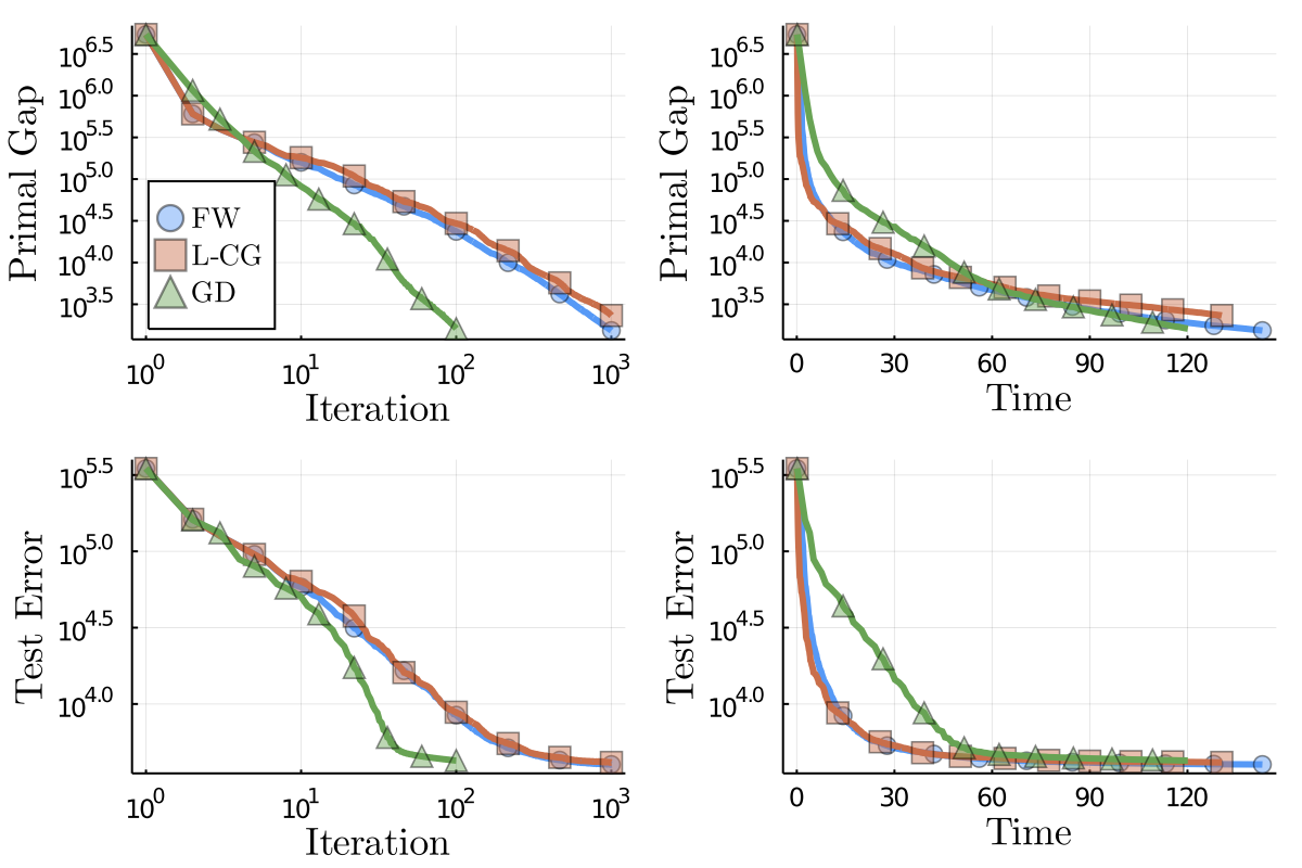
Figure 2. Movielens results.
The results are presented in Figure 2. We can clearly observe that the computational cost of a single PGD iteration is much higher than the cost of a FW variant step. The FW variants tested complete $10^3$ iterations in around $120$ seconds, while the PGD algorithm only completes $10^2$ iterations in a similar time frame. We also observe that the progress per iteration made by each projection-free variant is smaller than the progress made by PGD, as expected. Note that, minimizing a linear function over the nuclear norm ball, in order to compute the LMO, amounts to computing the left and right singular vectors associated with the largest singular value, which we do using the $\texttt{ARPACK}$ Julia wrapper in the current example. On the other hand, projecting onto the nuclear norm ball requires computing a full singular value decomposition. The underlying linear solver can be switched by users developing their own LMO.
The top two figures in Figure 2 present the primal gap of the matrix completion problem objective function in terms of iteration count and wall-clock time. The two bottom figures show the performance on a test set of entries. Note that the test error stagnates for all methods, as expected. Even though the training error decreases linearly for PGD for all iterations, the test error stagnates quickly. The final test error of PGD is about $6\%$ higher than the final test error of the standard FW algorithm, which is also $2\%$ smaller than the final test error of the lazy FW algorithm. We would like to stress though that the intention here is primarily to showcase the algorithms and the results are considered to be illustrative in nature only rather than a proper evaluation with correct hyper-parameter tuning.
Another key aspect of FW algorithms is the sparsity of the provided solutions. Sparsity in this context refers to a matrix being low-rank. Although each solution is a dense matrix in terms of non-zeros, it can be decomposed as a sum of a small number of rank-one terms, each represented as a pair of left and right vectors. At each iteration, FW algorithms add at most one rank-one term to the iterate, thus resulting in a low-rank solution by design. In our example here, the final FW solution is of rank at most $95$ while the lazified version provides a sparser solution of rank at most $80$. The lower rank of the lazified FW is due to the fact that this algorithm sometimes avoids calling the LMO if there already exists an atom (here rank-1 factor) in the cache that guarantees enough progress; the higher sparsity might help with interpretability and robustness to noise. In contrast, the solution computed by PGD is of full column rank and even after truncating the spectrum, removing factors with small singular values, it is still of much higher rank than the FW solutions.
Exact optimization with rational arithmetic
The package allows for exact optimization with rational arithmetic. For this, it suffices to set up the LMO to be rational and choose an appropriate step-size rule as detailed below. For the LMOs included in the package, this simply means initializing the radius with a rational-compatible element type, e.g., $\texttt{1}$, rather than a floating-point number, e.g., $\texttt{1.0}$. Given that numerators and denominators can become quite large in rational arithmetic, it is strongly advised to base the used rationals on extended-precision integer types such as $\texttt{BigInt}$, i.e., we use $\texttt{Rational{BigInt}}$. For the probability simplex LMO with a rational radius of $\texttt{1}$, the LMO would be created as follows:
lmo = FrankWolfe.ProbabilitySimplexOracle{Rational{BigInt}}(1)
As mentioned before, the second requirement ensuring that the computation runs in rational arithmetic is a rational-compatible step-size rule. The most basic step-size rule compatible with rational optimization is the $\texttt{agnostic}$ step-size rule with $\gamma_t = 2/(2+t)$. With this step-size rule, the gradient does not even need to be rational as long as the atom computed by the LMO is of a rational type. Assuming these requirements are met, all iterates and the computed solution will then be rational:
n = 100
x = fill(big(1)//100, n)
# equivalent to { 1/100 }^100
Another possible step-size rule is $\texttt{rationalshortstep}$ which computes the step size by minimizing the smoothness inequality as $\gamma_t = \frac{\langle \nabla f(\mathbf{x}_t), \mathbf{x}_t - \mathbf{v}_t\rangle}{2 L |\mathbf{x}_t - \mathbf{v}_t|^2}$. However, as this step size depends on an upper bound on the Lipschitz constant $L$ as well as the inner product with the gradient $\nabla f(\mathbf{x}_t)$, both have to be of a rational type.
Doubly stochastic matrices
The set of doubly stochastic matrices or Birkhoff polytope appears in various combinatorial problems including matching and ranking. It is the convex hull of permutation matrices, a property of interest for FW algorithms because the individual atoms returned by the LMO only have $n$ non-zero entries for $n\times n$ matrices. A linear function can be minimized over the Birkhoff polytope using the Hungarian algorithm. This LMO is substantially more expensive than minimizing a linear function over the $\ell_1$-ball norm, and thus the algorithm performance benefits from lazification. We present the performance profile of several FW variants in the following example on $200\times 200$ matrices. The results are presented in Figure 3.
The per-iteration primal value evolution is nearly identical for FW and the lazy cache variants. We can observe a slower decrease rate in the first 10 iterations of BCG for both the primal value and the dual gap. This initial overhead is however compensated after the first iterations, BCG is the only algorithm terminating with the desired dual gap of $10^{-7}$ and not with the iteration limit. In terms of runtime, all lazified variants outperform the standard FW, the overhead of allocating and managing the cache are compensated by the reduced number of calls to the LMO.
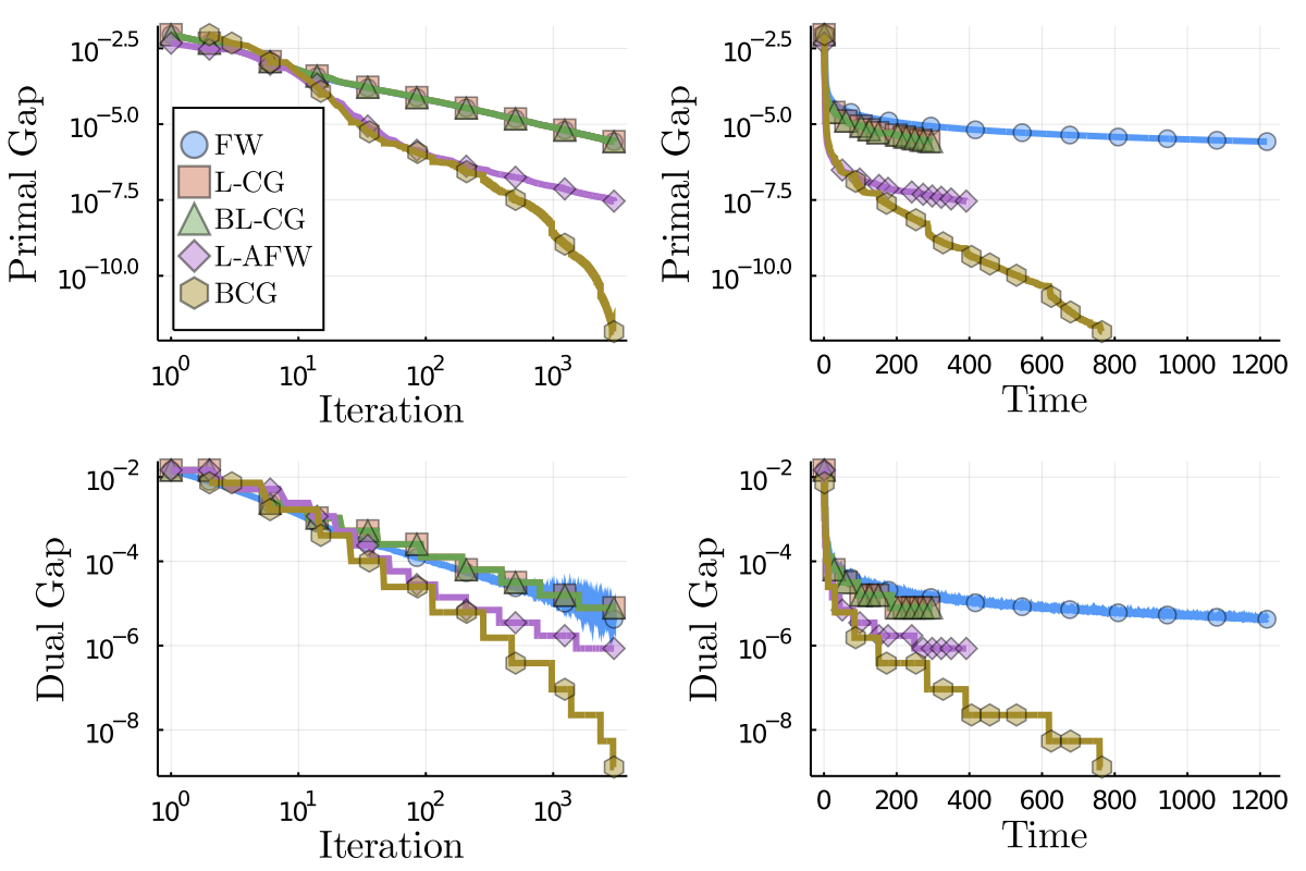
Figure 3. Doubly stochastic matrices results.
References
[FW] Frank, M., & Wolfe, P. (1956). An algorithm for quadratic programming. In Naval research logistics quarterly, 3(1-2), 95-110.
[LP] Levitin, E. S., & Polyak, B. T. (1966). Constrained minimization methods. In USSR Computational mathematics and mathematical physics, 6(5), 1-50.
[CP] Combettes, C. W., & Pokutta, S. (2021). Complexity of linear minimization and projection on some sets. In arXiv preprint arXiv:2101.10040. pdf
[BCP] Besançon, M., Carderera, A., & Pokutta, S. (2021). FrankWolfe.jl: a high-performance and flexible toolbox for Frank-Wolfe algorithms and Conditional Gradients. In arXiv preprint arXiv:2104.06675. pdf
[GM] Guélat, J., & Marcotte, P. (1986). Some comments on Wolfe’s ‘away step’. In Mathematical Programming 35(1) (pp. 110–119). Springer. pdf
[LJ] Lacoste-Julien, S., & Jaggi, M. (2015). On the global linear convergence of Frank-Wolfe optimization variants. In Advances in Neural Information Processing Systems 2015 (pp. 496-504). pdf
[BPZ] Braun, G., Pokutta, S., & Zink, D. (2017). Lazifying Conditional Gradient Algorithms. In Proceedings of the 34th International Conference on Machine Learning. pdf
[BPTW] Braun, G., Pokutta, S., Tu, D., & Wright, S. (2019). Blended conditonal gradients. In International Conference on Machine Learning (pp. 735-743). PMLR. pdf
[HL] Hazan, E. & Luo, H. (2016). Variance-reduced and projection-free stochastic optimization. In Proceedings of the 33rd International Conference on Machine Learning. pdf
[PNAM] Pedregosa, F., Negiar, G., Askari, A., & Jaggi, M. (2020). Linearly Convergent Frank-Wolfe with Backtracking Line-Search. In Proceedings of the 23rd International Conference on Artificial Intelligence and Statistics. pdf
Comments